Download
1 / 24
240 likes | 264 Views
Anvendt Spektroskopi Applied Spectroscopy KJM3000 Høst 2018. Curriculum : - ” Introduction to Spectroscopy ” by Pavia , Lampman , Kriz , Vyvyan All lecture notes All problem sets. Practical information. Lecturer: Tore Bonge-Hansen, rom Ø301, torehans@kjemi.uio.no

E N D
Anvendt Spektroskopi Applied Spectroscopy KJM3000 Høst 2018 Curriculum : - ”Introduction to Spectroscopy” by Pavia, Lampman, Kriz, Vyvyan • All lecture notes • All problem sets
Practical information Lecturer: Tore Bonge-Hansen, rom Ø301, torehans@kjemi.uio.no Lectures and problems: Berzelius, Wed 10.15 Curie, Thu 12.15 Communication: e-mail and homepage. No Canvas! 80% of the problemsets must be approved/passed in order to take the exam. No grade on the problemsets.
Goal : The student should be able to use spectroscopic methods to determine the constitution of organic molecules. Plan: ca. 20 hours of lectures and ca. 40 hours problem solving. Less focus on theory, more on solving problems. Last problem: Thu 29/11. Exam: 20/12. 4h written exam, letter grade. Four spectroscopic methods : UV/VIS, IR, NMR og MS. These methods give complementary info, and together they are a a very powerful tool for identification and structure elucidation of small amounts (mg) of unknown compounds.
KJM1110 (Org 1) exam 2017 MF: C7H12O3 IR: 1723 and 1733
NMR-spectroscopyKjernemagnetisk resonans • History • Physical requirements • Principles • Theory • Interpretation of spectra
History • 1946: NMR discovered • 1949: Chemical shift • 1953: First commercial high resolution instrument • 1960: Structure determination of organic molecules • 1970: FT-NMR • 1971 – 75 : 2D-NMR • 1973: MR-tomography
Physical requirements 1.Nuclear spin (12C and 16O are NMR silent) Magnetic moment 2. Magnetic field Number of spin states in the presence of a magnetic field = 2I +1 1H and 13C # spin states = 2 2H # spin states = 3
ΔE = hν ν = γB0/2π ν = frequency, B0 = applied magnetic field, γ = magnetogyric ratio
N1 = number of nuclei in the α state N2 = number of nuclei in the β state N1/N2 is given by Boltzmann’s distribution: At 60 MHz: excess in α state is 9 nuclei in a population of 2 million. The N1/N2 ratio increases with increasing B0.
δ-scale Tetramethylsilane, Si(Me)4 is used as reference in both 1H and 13C TMS: - The nuclei are strongly shielded and appear to the right - 12 1H and 4 13C nuclei - One singel peak - Chemically inert - Non toxic
Integration CW(1H): The area is proportional to the number of nuclei in the peak FT(1H): Same as CW given that the relaxtion time is long enough (2-3 s) FT(13C): Not commonly used due to slow relaxtion and large difference in relaxtion rates for different 13C nuclei.