Download
1 / 38
380 likes | 629 Views
Ch.7 The Capital Asset Pricing Model: Another View About Risk. 7.1 Introduction 7.2 The Traditional Approach to the CAPM 7.3 Using the CAPM to value risky cash flows 7.4 The Mathematics of the Portfolio Frontier: Many Risky Assets and No Risk-Free Asset

E N D
Ch.7 The Capital Asset Pricing Model: Another View About Risk • 7.1 Introduction • 7.2 The Traditional Approach to the CAPM • 7.3 Using the CAPM to value risky cash flows • 7.4 The Mathematics of the Portfolio Frontier: Many Risky Assets and No Risk-Free Asset • 7.5 Characterizing Efficient Portfolios -- (No Risk-Free Assets) • 7.6 Background for Deriving the Zero-Beta CAPM: Notion of a Zero Covariance Portfolio • 7.7 The Zero-Beta Capital Asset Pricing Model • 7.8 The Standard CAPM • 7.9 Conclusion
7.1 Introduction • Equilibrium theory (in search of appropriate risk premium) • Exchange economy • Supply = demand: for all asset j, • Implications for returns
7.2 The Traditional Approach • All agents are mean-variance maximizers • Same beliefs (expected returns and covariance matrix) • There exists a risk free asset • Common linear efficient frontier • Separation/ Two fund theorem • T = M
(7.1) 7.2 The Traditional Approach to the CAPM • a. The market portfolio is efficient since it is on the efficient frontier. • b. All individual optimal portfolios are located on the half-line originating at point . • c. The slope of the CML is .
Proof of the CAPM relationship (Appendix 7.1) • Refer to Figure 7.1. Consider a portfolio with a fraction 1- a of wealth invested in an arbitrary security j and a fraction a in the market portfolio As a varies we trace a locus which - passes through M (- and through j) - cannot cross the CML (why?) - hence must be tangent to the CML at M Tangency = = slope of the locus at M = slope of CML =
(7.2) (7.3) Define Only a portion of total risk is remunerated = Systematic risk
(7.4) (7.5) A portfolio is efficient iff no diversifiable risk (7.6) b is the only factor; SML is linear
7.4 The Mathematics of the Portfolio Frontier: Many Risky Assets and No Risk-Free Asset Goal: understand better what the CAPM is really about – In the process: generalize. • No risk free asset • Vector of expected returns e • Returns are linearly independent • Vij = sij
Definition 7.1: A frontier portfolio is one which displays minimum variance among all feasible portfolios with the same . since
(vector) (vector) l (scalar) g (scalar) (7.15) (vector) (vector) (scalar) If E = 0, wp = g If E = 1, wp = g + h
Proposition 7.1: The entire set of frontier portfolios can be generated by ("are convex combinations" of) g and g+h. • Proof: To see this let q be an arbitrary frontier portfolio with as its expected return. Consider portfolio weights (proportions) ; then, as asserted,
. • Proposition 7.2. The portfolio frontier can be described as convex combinations of anytwo frontier portfolios, not just the frontier portfolios g and g+h. • Proof: To see this, let be any two distinct frontier portfolios; since the frontier portfolios are different, Let q be an arbitrary frontier portfolio, with expected return equal to . Since , there must exist a unique number such that (7.16) Now consider a portfolio of with weights a, 1- a, respectively, as determined by (7.16). We must show that .
(7.17) • For any portfolio on the frontier, , with g and h as defined earlier. Multiplying all this out yields:
(i) the expected return of the minimum variance portfolio is A/C; • (ii) the variance of the minimum variance portfolio is given by 1/C; • (iii) equation (7.17) is the equation of a parabola with vertex (1/C, A/C) in the expected return/variance space and of a hyperbola in the expected return/standard deviation space. See Figures 7.3 and 7.4.
Figure 7-3 The Set of Frontier Portfolios: Mean/Variance Space
Figure 7-5 The Set of Frontier Portfolios: Short Selling Allowed
7.4 Characterizing Efficient Portfolios -- (No Risk-Free Assets) • Definition 7.2: Efficient portfolios are those frontier portfolios for which the expected return exceeds A/C, the expected return of the minimum variance portfolio.
Proposition 7.3 : Any convex combination of frontier portfolios is also a frontier portfolio. • Proof : Let , define N frontier portfolios ( represents the vector defining the composition of the ith portfolios) and let , i = 1, ..., N be real numbers such that . Lastly, let denote the expected return of portfolio with weights . The weights corresponding to a linear combination of the above N portfolios are : Thus is a frontier portfolio with .
Proposition 7.4 : The set of efficient portfolios is a convex set . • This does not mean, however, that the frontier of this set is convex-shaped in the risk-return space. • Proof : Suppose each of the N portfolios considered above was efficient; then , for every portfolio i. However ; thus, the convex combination is efficient as well. So the set of efficient porfolios, as characterized by their portfolio weights, is a convex set.
7.5 Background for Deriving the Zero-Beta CAPM: Notion of a Zero Covariance Portfolio • Proposition 7.5: For any frontier portfolio p, except the minimum variance portfolio, there exists a unique frontier portfolio with which p has zero covariance. We will call this portfolio the "zero covariance portfolio relative to p", and denote its vector of portfolio weights by . • Proof: by construction.
E ( r ) p A/C MVP ZC(p) E[r ( ZC(p)] (1/C) Var ( r ) Figure 7-6 The Set of Frontier Portfolios: Location of the Zero-Covariance Portfolio
Let q be any portfolio (not necessary on the frontier) and let p be any frontier portfolio. (7.27)
7.6 The Zero-Beta Capital Asset Pricing Model (Equilibrium) (i) agents maximize expected utility with increasing and strictly concave utility of money functions and asset returns are multivariate normally distributed, or (ii) each agent chooses a portfolio with the objective of maximizing a derived utility function of the form , W concave. (iii) common time horizon, (iv) homogeneous beliefs about e and V
(7.28) (7.29) • All investors hold mean-variance efficient portfolios • the market portfolio is convex combination of efficient portfolios is efficient. • (7.21) .
(7.30) n x 1 n x n a number n x 1 7.7 The Standard CAPM Solving this problem gives
(7.31) (7.32) (7.33)
(7.34) or (7.35) or
What have we accomplished? • The pure mathematics of the mean-variance portfolio frontier goes a long way • In particular in producing a SML-like relationship where any frontier portfolio and its zero-covariance kin are the heroes! • The CAPM = a set of hypotheses guaranteeing that the efficient frontier is relevant (mean-variance optimizing) and the same for everyone (homogeneous expectations and identical horizons)
What have we accomplished? • The implication: every investor holds a mean-variance efficient portfolio • Since the efficient frontier is a convex set, this implies that the market portfolio is efficient. This is the key lesson of the CAPM. It does not rely on the existence of a risk free asset. • The mathematics of the efficient frontier then produces the SML
What have we accomplished? • In the process, we have obtained easily workable formulas permitting to compute efficient portfolio weights with or without risk-free asset
Conclusions • The asset management implications of the CAPM • The testability of the CAPM: what is M? the fragility of betas to its definition (The Roll critique) • The market may not be the only factor (Fama-French) • Remains: do not bear diversifiable risk!