GEO-CAPE Science Team Meeting May 21-24, 2013 NASA Ames Research Center

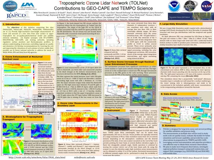
1. Tropospheric Ozone Lidar Network (TOLNet) Contributions to GEO-CAPE and TEMPO Science Mike Newchurch1, Jassim A. Al-Saadi2,3, Raul J. Alvarez4, John Burris5, Wesley Cantrell1, GaoChen3, Russell DeYoung3, R. Michael Hardesty4, Jerry Herwehe6, Guanyu Huang1, Raymond M. Hoff7, Jack A. Kaye2, Shi Kuang1, Kevin Kunpp1, Andy Langford4, Thierry Leblanc8, Stuart McDermid8, Thomas J. McGee5, R. Bradley Pierce9, Christopher J. Senff4, John Sullivan7, Jim Szykman4, Gail Tonnesen4, Lihua Wang1 1UAHuntsville,2NASA/HQ, 3NASA/LaRC, 4NOAA/ESRL, 5NASA/GSFC, 6USEPA,7UMBC ,8NASA/JPL, 9NOAA/NESDIS The ozone retrievals from three lidar channels (2 independent receivers ) are consistent each other with an average bias less than 10% in their retrievable altitude ranges. All three channels’ retrievals show the ozone transition from ~80-~55 ppbv below 1 km at 21:00. The retrievals of the 3 channels with 10-min integration time at 13:09 agree with the ozonesonde profile at 13:10 to within several percent. These errors primarily arise from uncertainties originating with the signal processing, including the solar background correction, SIB correction, choice of the average signal integration interval/time, and signal smoothing using numerical filters. In Figure 2, the hook-shaped low RH stream outlines the trajectory where the dry stratospheric air ‘leaked’ into the troposphere. The shape of the high IPV on the 320-K Θ surface associated with the cutoff low agrees perfectly with the RH distribution. The jet stream was just located above Huntsville with a maximum wind speed exceeding 60 m/s. 7. Large-Eddy Simulation The objectives of this initiative comprising five sites (NASA/GSFC, NASA/LaRC, NASA/JPL, NOAA/ESRL, UAHuntsville) are to (1) Provide high-resolution time-height measurements of ozone and aerosols at a few sites from near surface to upper troposphere for air-quality/photochemical model and satellite retrieval validation; (2) Exploit synergies with EV-I/TEMPO, DISCOVER-AQ, GEO-CAPE, and existing networks, including regulatory surface monitors and thermodynamic profilers, to advance understanding of processes controlling regional air quality and chemistry; (3) Develop recommendations for lowering the cost and improving the robustness of such systems to better enable their possible use in future national networks to address the needs of NASA, NOAA, EPA and State/local AQ agencies. 1. Introduction We use a Large-Eddy Simulation model coupled with a photochemical package (LES-Chem), developed by Dr. Jerry Herwehe, to simulate PBL structure and trace gas distributions with fine temporal and spatial resolution.. An ideal afternoon PBL case simulated by LES-Chem in Figure 8. The grid cell volume is 50m * 50m * 50m in a 10km* 10 km *4km domain with no mean large-scale wind and with a uniformly-heated bottom surface in order to produce pure convection, initialized with a midday boundary layer depth of around 2 km AGL. 539ppbv at 9.6km 150ppbv at 6.5km 320ppbv at 8km (a) Cloud Cloud Cloud Figure 5. Ozone lidar retrieval compared with the ozonesonde and EPA (~16 km away )surface measurements (Kuang et al., 2013). (b) 2. Ozone Enhancement at Nocturnal Residual Layer 5. Surface Ozone Increase through Residual Layer Entrainment Processes Figure 1.An ozone enhancement in the nocturnal residual layer was observed by the UAHuntsvilleozone lidar from the late evening to midnight on 4 October 2008. The ozone enhancement is due to the Low-level jet. The surface ozone enhancement at Oct. 5 can be explained by the high ozone at residual layer at previous day (Kuang et al., 2011). (a) UAH O3 DIAL measurements with 10-min resolution The entrainment processes have significant contributions on either ozone maxima or rapid ozone enhance during the next day. The high- ozone air in the residual layer is mixed into PBL through entrainment processes as the PBL grows in the early morning. These processes may account 60-70% of the daytime surface ozone maxima. 302K Figure 3. Local measurements of the 27-29 April 2010 STT event in Huntsville. (a) Ozone lidar and ozonesonde (marked by the black triangle at the bottom) measurements; (b) Θ structures derived from the MPR. (Kuang et al., 2012) . Figure 8. The left panel represents a X-Y horizontal slice, at the entrainment zone (about 2000 m AGL), showing the most vigorous thermals (with tracer) punching into the inversion at the top of the PBL. The right panel represents a 3-D view of the mature convective mid-day PBL containing the tracer (Herwehe 2002) (b) Co-located ceilometer backscatter The lidar captures the initial intrusion ‘nose’ with 150-ppbv ozone at 6.5 km at ~1600 27 April and thereafter a distinct descending high ozone belt with a thickness of ~1-2-km after the major intrusion tongue body exited the Huntsville upper air. The high ozone layer between 70 and 85 ppbv at Θ=302-310 K at ~7km at 3000 29 April, which sank from higher Θ surface (>320 K), descent to the ~298-K Θ surface at ~2.5 km at 0615 with a rate of ~4 km/day. Another important variation is that the upper tropospheric ozone of ~60-70 ppbv above the STT layer before 1800 decreased to ~40-50 ppbvdue to mixing of the low ozone air from the west. This simulation shows that a purportedly “well-mixed” afternoon boundary layer is actually not well-mixed for a surface-emitted gas; the tracer mixing ratio is inhomogeneous and tends to be concentrated in the turbulent updrafts, with lesser concentrations in the compensating subsidence around the thermals. . 8. Data Access Figure 6. Surface ozone rapid increase in the early morning measured by a tethered balloon (left panel). The right panel shows simultaneous and co-located observations by ceilometer (Huang et al., in prep.). http://www-air.larc.nasa.gov/missions/TOLNet/ or http://nsstc.uah.edu/atmchem/lidar/DIAL_data.html Low-level jet Low-level jet 4. Ozone Lidar Measurements in the Boundary Layer (c) Co-located 915-MHz wind profiler (c) Co-located 915-MHz wind profiler 6. Instrument Figure 7. Truck-based, scanning NOAA/ESRL TOPAZ lidar at the 2012 Uintah Basin study. TOPAZ (Tunable Optical Profiler for Aerosol and oZone) lidar is a state-of-the-art, compact differential absorption lidar (DIAL) for measuring ozone profiles with high temporal and spatial resolution (Alvarez et al., 2011). (d) EPA surface O3 and CBL height 3. Stratosphere-to-Troposphere Transport (a) (b) 9. Summary Cutoff low TOLNet is designed for long-term ozone and aerosol profiling for satellite validation and process study. The measurements at multiple sites will be used to study multi-scale air-quality issues, evaluate AQ models for better simulation and forecast capability, and provide fine-scale observations in preparation for TEMPO and GEO-CAPE. Leveraging current instrumentation and expertise provides a cost-effective way to obtain these research observations. We plan to make more frequent observations, investigate regional pollution transport using multi-station data, and support field campaigns (e.g. DISCOVER-AQ and SEAC4RS) with mobile lidar. Huntsville The instrument is based on a Nd:YLF pumped Ce:LiCAF ultraviolet laser. TOPAZ emits three wavelengths, that can be tuned from approximately 283 nm to 310 nm. Ozone profiles are typically retrieved at a range resolution of 90 m. Time resolution varies from 10 s to several minutes depending on the atmospheric conditions and the desired precision of the data. A two-axis scanner mounted on the roof of the truck permits pointing the laser beam at several shallow elevation angles at a fixed, but changeable azimuth angle. Zenith operation is achieved by moving the scanner mirror out of the laser beam path. By using the scanner to vary the elevation angle, high resolution ozone measurements can be obtained to within 15 m of the surface. Horizontal measurements at different azimuth angles can be performed to study the variability of ozone near the surface. (c) Figure 2. Horizontal distributions of (a) wind speed and RH at 300hPa at 1200 UTC; (b) IPV at 320-K isentropic surface with a 2-PVU interval and the 2-PVU based tropopause pressure at 1200 UTC; (c) OMI total ozone, on 27 April 2010(Kuang et al., 2012) Figure 4. Ozone lidar retrievals (Channel 1 – bottom, Channel 2 – middle, and Channel 3 - top) compared with ozonesonde (marked by the black triangle at 13:10 launch time) and EPA (~ 16 km away from lidar station) hourly surface measurements (Kuanget al., 2013). GEO-CAPE Science Team Meeting May 21-24, 2013 NASA Ames Research Center http://nsstc.uah.edu/atmchem/lidar/DIAL_data.htmlmike@nsstc.uah.edu