Download

1 / 30
300 likes | 493 Views
Fig. 7 Repeated generations of self-fertilization will eventually split a heterozygous population into a series of completely homozygous lines. The rate of loss of heterozygosity per generation in inbreeding H t = H 0 ( 1 - 1/ 2 N ) t H 0 e -t/2N

E N D
Fig. 7 Repeated generations of self-fertilization will eventually split a heterozygous population into a series of completely homozygous lines
The rate of loss of heterozygosity per generation in inbreeding Ht = H0 ( 1 - 1/ 2N)t H0e-t/2N 2N : the total number of haploid genomes N : the number of diploid individuals in the population Ht : the proportions of heterozygotes in the tth H0 : the proportions of heterozygotes in the original generation t , Ht 0 각 유전자마다 ½씩 heterozygosity 감소 Balance between inbreeding and new variation In nature, the actual variation available for natural selection is a balance between the introduction of new variation and its loss through local inbreeding (1/2N) new variation 1/2N (loss of heterozygosity)
A A a
P값에 상관없음 Delta P = pq(WA bar –Wa bar)/W bar WA bar = pWA/A + qWA/a Completely deleterious allele q = 1-s =root (u/s) Deletorious gene with some effect on heterozygoyes WA/A = 1.0, WA/a = 1-hs, Wa/a = 1-s h = degree of dominance of the deleterious allele qcap = u/hs
Chapter 25. Quantitative genetics • Key concept • In natural populations, the variation is quantitative, not qualitative. • 2. Mendelian genetic analysis is extremely difficult to apply to such continuous phenotypic distributions: statistical technique are employed. • 3. A major task: to determine the ways in which genes interact with the environment -> the formation of a given quantitative trait distribution. • 4. The genetic variation underlying a continuous character distribution = 1) segregation at a single genetic locus or 2) at numerous interacting loci that produce cumulative effect on the phenotype. • 5. The estimated ratio of genetic to environmental variation is not a measure of the relative contribution of genes and environment to phenotype; Estimates of genetic and environmental variance are specific to the single population and the particular set of environments.
Goal of genetics The analysis of the genotype of organisms; can be identified only through phenotypic effect. Actual variation between organisms is usually quantitative, not qualitative. height, weight, shape, color, metabolic activity, reproductive rate, behavior vary continuously over a range. (figure 25-1) ex) corn plant cross between 8 feet tall and 3 feet tall continuously distributed in height Continuity of phenotype is the result of two phenomena. 1. Each phenotype does not have norm of reaction. 2. Many loci may have alleles that make a difference in the phenotype under observation. Many different genotypes may have the same average phenotype. Two individuals of the same genotype may not have same phenotype <- environmental variation.
Quantitative genetics : the study of the genetics of continuously varying characters. 교재 745쪽 Some basic statistical notions 1. Distributions Mendelian character description: proportions of the offspring that fall into several distinct phenotypic classes or often simply the presence or absence of a class. Quantitative character description: basic concept is that of the statistical distribution. Frequency histogram; ( figure 25-2a) a graph of numbers of individuals observed against measurement class Distribution functionof heights in the population: continuos appearance as of Figure 25-2c.
<Figure 25-2> Frequency distribution for height of males: (a) a histogram with 5-cm class intervals; (b) a histogram with 1-cm class intervals; c) the limiting continuous distribution.
Some basic statistical notions 2. Statistical measures • 1. Need a measure of central tendency • 2. Need a measure of dispersion • 3. Need a measure of relation between measurements. • The most commonly used measures of central tendency: • mode ( the most frequent observation ) • mean ( arithmetic average of the observation) • The dispersion of a distribution: measured by the variance • The relation between different variables: measured by their correlation -> see Statistical appendix in 764 page - measures central tendency: mode and mean - measures of dispersion: variance - measures of relation: covariancen and correlation covariance and variance of sum, regression, samples and populations
Genotypes and phenotypic distribution • using the concept of distribution, mean, and variance • understanding the difference between quantitative and mendelian genetic trait. <Figure 25-3> (a) Phenotypic distributions of three genotypes. (b) A population phenotypic distribution result from mixing individuals of the three genotypes in a proportion 1:2:3 (a/a, A/a, A/A) Two features of the total distribution 1) there is only a single mode. (despite of three separate genotypic distribution, population distribution does not reveal the separate mode) 2) any individual whose height lies between the two arrows could have come from any one of three genotypes, because they overlap so much. can not perform mendelian analysis
<Figure 25-4> when the same genotypes as those in figure 25-3 are grown in carefully controlled stress environments, the result is a smaller phenotypic variation in each genotype and a greater difference between genotypes. The height of the individual distribution in part b are proportional to the frequencies of the genotypes in the mixture. Multiple factor hypothesis: basic model of quantitative genetics - large numbers of genes, each with a small effect, are segregating to produce quantitative variation. (polygenes) - Number of segregating loci that influence a trait is not what separate quantitative and qualitative characters. - Johansen`s experiment: 1. produced 19 homozygous lines by inbreeding of bean plants 2. seed weight (0.35g-0.64g), quantitative distribution 3. It takes only a few genetically varying loci to produce variation that is indistinguishable from the effect of many loci of small effect. (if 5 loci with 3 alleles, 243 different kinds of homozygotes) -> 1. There is no dividing line between polygenic traits and other traits. 2. No phenotypic trait above the level of aa sequence in a polypeptide is influenced by only one gene. 3. Some genes will have major effect on a trait; others, minor effects.
Norm of reaction and phenotypic distribution • The phenotypic distribution of a trait • function of average differences between genotypes • function of the variation between genotypically identical individuals • Both are functions of the sequence of environment. • Distribution of environment will be reflected biologically as a distribution of phenotypes determined by norm of reaction < Fig.> The distribution of environment on the horizontal axis is converted into the distribution of phenotypes on the vertical axis by the norm of reation of a genotype. Frequency distribution of phenotypes The frequency distribution of developmental environments will be reflected as a frequency distribution of phenotypes as determined by the shape of the norm of reaction curve. # of individual The symmetric environmental distribution is converted into an asymmetric phenotype distribution with a long tail at the larger plant heights, corresponding to the lower temperature.
<Fig. 25-6> Two different environmental distribution are converted into different phenotypic distributions by two genotypes. Environments at black distribution curve --> population of plants have unimodal distribution. Environment is shifted to the right --> bimodal distribution of phenotypes
Determining norms of reaction Llittle is known about the norm of reaction for any quantitative trait in any species. --> because it is difficult in most sexually reproducing species to replicate a genotype, it can be tested in different environment. In domesticated plants and animals - A few norm of reaction studies carried out with plants that can be clonally propagated. - By mating close relatives or inbreeding, a segregating line (contain both homozygote and heterozygote )can be made homozygous. - The purpose of creating homozygous lines: to develop in different environment to produce a norm of reaction. - For norm of reaction study, all the individuals should be absolutely identical. - The process of inbreeding increases the homozygosity of the group slowly. Hetn = 1/2n x Het0 Hetn : the proportion of heterozygous loci in the nth generation Het0 :the proportion in the 0 generation Selfing of Aa -> ½ homozygotes
Determining norms of reaction In natural populations • Each inbred line can be crossed to every other inbred line to produce heterozygotes • that reconstitute the original population. C; crossover suppressor l; recessive lethal M1, M2; dominant marker <Fig. 25-7> Method for making autosomes homozygous by using dominant marker genes M1 and M2, a crossover suppressor C, and a lethal gene I
Determining norms of reaction Results of norm of reaction studies <Fig. 25-8> The number of abdominal bristles in different homozygous genotypes of Drosophila Pseudoobscura at three temparature. 1. Norm of reaction studies show only small differences between natural genotypes, and these differences are not consistent over a wide range of environments. 2. “superior” genotypes in domesticated animals and cultivated plants may be superior only in certain environments. 3. If it should turn out that humans exhibit genetic variation for various mental and emotional traits, this variation is unlikely to favor one genotype Over another across a range of environments. <Fig. 25-9> Yields of grain two varieties of corn in Different environments (a)at a high plating density (b) at a low plating density - variety 1 : older variety of hybrid corn variety 2 : later improved hybrid - at high density : new variety is clearly superior. at low density : new is less sensitive environment new is poorer under the best farm condition.
Heritability of a trait The question of whether a trait is heritable is a question about the role that differences in genes between individuals or groups. Familiality and heritability - Traits are familial if members of the same family share them. - Traits are heritable only if the similarity arises from shared genotypes. - Two general methods for establishing the heritability of a trait: 1) phenotypic similarity between relatives 2) using marker gene segregation; genotypes carrying different alleles of marker gene also differ in their average phenotype for the quantitative character - Marker loci can be observed electroporetic studies of protein variation or immunological study - DNA sequence variation detected by gain or loss of sites of cleavage of restriction enzyme; RFLP.
Heritability of a trait Phenotypic similarity between relatives In experimental organisms, environmental similarity can often be readily distinguished from genetic similarity(heritability). In humans,however, it is very difficult to determine whether a particular trait is heritable. <Fig. 25-10> standard method for testing heritability in experimental organisms.
Quantifying heritability Two part of total phenotypic variance of the population (Sp2): - the variance between genotypic means (Sg2) genetic variance - the remaining veriance(Se2) environmental variance • - If the phenotype is the sum of genetic and an environmental effect, P=G+E, • the variance of the phenotype is the sum of the genetic variance, twice the covariance between • the genotype and environmental effects. • Sp2 =Sg2 +Se2 + 2cov ge • The degree of heritability can be defined as the part of the total variance that is due to genetic • variance. • H2 = Sg2 /Sp2 =Sg2 /Sg2+ Se2 • - H2 is called the broad heritability of the character Analysis of variance
Quantifying heritability Method of estimating H2 Estimation of genetic variance and heritability • - Directly, obtain an estimate of Se2 by making a number of homozygous lines from the population, crossing them in pairs to reconstitute individual homozygotes, and measuring the phenotypic variance within each heterozygote genotype. • - Considering the genetic similarities between relatives: • Averaging over their paternally and maternally inherited genes, half the genes of full • siblings are identical between them. • Their genetic correlation, which is equal to the chance that carry the same allele, is 1/2 . • (genetic correlation of full siblings) - (genetic correlation of half-sibling) = 1/4 • but • (phenotypic correlation of full-siblings) - (phenotypic correlation of half-siblings) • = H2 x 1/4 • H2 = 4[(correlation of full-siblings) - (correlation of half-siblings)] • (correlation here is phenotypic correlation) • - Genetic similarities between parents and offspring and between twins to obtain to H2 • H2 = 4(correlation of full-sibling) - 2(parent-offspring correlation ) • H2 = 2 [(correlation of monozygotic twins) - (correlation of dizygotic twins)] It is just a estimation of heritability!
Quantifying heritability Children Biological parents Adoptive parents 110 90 118 112 92 114 114 94 110 116 96 120 118 98 112 120 100 116 115 95 115 mean Meaning of H2 1. If there is a nonzero heritability in the population and in the environments in which the organisms have developed, genetic differences have influenced the variation between individuals, so genetic differences do matter to the trait. 2. The value of the H2 provide a limited prediction of the effect environmental modification under particular circumstances. - Example of the erroneous use of heritability arguments ( human IQ performance and social success ) • Children have a high correlation • with their biological parents. • However , the mean IQ of the • children is equal to the mean IQ of • the adoptive parents. • - Heritability is not the opposite of phenotypic plasticity. • A character may have perfect heritability in a population and still be • subject to great changes resulting from environmental variation.
Quantifying heritability Locating the genes • - Genetic analysis detects genes only when there is some allelic variation. • Molecular analysis can identify genes even when they do not vary: the gene products can be • identified. • - It is sometimes possible to use knowledge of the biochemistry and development of organism to • guess that variation at a known locus is responsible for at least some of the variation in phenotypes. • - Example: variation in activity of the enzyme acid phosphatase in human RBC. < Fig. 25-11> Red cell acid phosphatase activity of different genotypes and the distribution of activity in an English population made up of a mixture these genotypes. Of the variance in activity in the total distribution (607.8), about half is explained by the average variance within genotypes(310.7) So half (607.8 - 310.7 = 297.1) is accounted for by the variance between the means of six genotypes.
Quantifying heritability Marker gene segregation • - The genes segregating for a quantitative trait, quantitative trait loci (QTLs), cannot be • individually identified in most cases. • - It is possible to localize those regions of the genome in which the relevant loci lie and • to estimate how much of the total variation is accounted for by QTL variation in each • region. • Analysis method: crossing two lines that differ markedly in the quantitative trait and • differ in alleles at well-known loci, marker genes: electronic mobility of the protein Linkage analysis • An experimental protocol for localizing the genes uses groups of individuals that differ • markedly in the quantitative trait and differ at marker loci. • A marker loci that is unlinked or very loosely linked to any QTLs will have the same • average value of the quantitative trait for all its genotypes. • One that is closely linked to some QTLs will differ in its mean phenotype from one • of its genotypes to another.
There are 4 unit of difference between the • average gamete carrying M and m allele in the • segregating F2. • - 8 unit of the difference between the two original • homozygous line. • 8 percent of the average difference between the • lines, although the QTLs actually account for 10 • percent of the difference. • - The discrepancy comes from the recombination • between the marker gene and the QTLs. • This technique used to locate chromosomal • segment associated with traits. <Fig. 25-12> Result of a cross between two selected lines that differ at a QTLs and in a molecular marker 10 crossover unit away from the QTLs. The QTL + allele adds 5 unit to the phenotype.
<Fig. 25-13> Distribution of associations of the traits differences between two lines of maize with an array of DNA markers. • Note that 55% of all the associations account for less than 1) of their trait differencens. • The attempt to map QTLs for human traits have not very successful, although the • segregating marker technique has been a success in finding loci whose mutations • are responsible for single-gene disorders.
More on analyzing variance The genetic variation and the environmental variation can themselves each be further subdivided to provide information about gene action and the possibility of shaping the genetic composition of a population. Additive and dominance variance • - For many quantitative traits, neither dominance nor no-dominance is the rule. • - In some case, heterozygotic phenotype may lie outside the phenotypic range of the homozygous • altogether (overdominance) • ex) newborn babies who are intermediate in size have higher chance of survival. • Additive genetic variation(Sa2): The variance that arises because there is an average difference • between the carrier of a alleles and the carriers of A alleles. • Dominance variance (Sd2): results from that heterozygotes are not exactly intermediate between • monozygotes. • Sg2 = Sa2 + Sd2 • Total phenotype variance • Sp2 = Sg2 + Se2 = Sa2 +Sd2 + Se2 • The heritability in the narrow sense (h2) • h2 = Sa2 / Sp2 = Sa2 / Sa2+ Sd2+ Se2 The effect of selection depends on the amount of additive genetic variance and not on the genetic variance in general. h2, not H2, is relevant for a prediction of response to selection.
More on analyzing variance Estimating genetic variance components < Fig. 25-15> Ranges of heritabilities (h2) reported for a variety of characters in chickens. <Fig. 25-14> The regression(red line), of offspring measurements (y)on midparents(x) for a trait with narrow heritability(h2) of 0.5. The blue line would be regression slope if the traits were perfectly heritable. • Selection differential: the difference between the • selected parents and the unselected mean. • selection response: the difference between their • offspring and the preceding generation. • - Selection response = h2 x selection differential • - h2 = selection response / selection differential
More on analyzing variance Use of h2 in breeding • - The subdivision of genetic variation and environmental variation provides important • information about gene action that can be used in plant and animal breeding. • - The higher h2 is, the higher parent-offspring correlation is. • If h2 is very low, H2 together with h2 can be of use to the breeder. • If h2 and H2 are both low; • - some scheme of reducing Se2 must be used. • - rather than choosing the best individuals, use family selection. • - If h2 is low but H2 is high, there is not much environmental variance; the low h2 is • the result of a small amount of additive genetic variance compared with dominance • and interaction variance. • - Hybrid-inbred method; corn (pure inbreds -> hybrid -> select the best one)