Download
1 / 35
370 likes | 557 Views
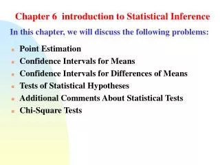
Chapter 6 introduction to Statistical Inference. In this chapter, we will discuss the following problems:. Point Estimation Confidence Intervals for Means Confidence Intervals for Differences of Means Tests of Statistical Hypotheses Additional Comments About Statistical Tests

E N D
Chapter 6 introduction to Statistical Inference In this chapter, we will discuss the following problems: • Point Estimation • Confidence Intervals for Means • Confidence Intervals for Differences of Means • Tests of Statistical Hypotheses • Additional Comments About Statistical Tests • Chi-Square Tests
6.1 Point Estimation In this chapter we develop statistical inference (estimation and testing) based on likelihood methods. We show that these procedures are asymptotically optimal under certain conditions. Suppose that X1, …, Xn~ (iid) X, with pdf f (x; ), (or pmf p(x; )), . 6.1.1The Maximum Likelihood Estimation The parameter (can be vectors) is unknown. The basis of our inferential procedures is the likelihood function given by, (6.1.1) L( ; x) = wherex = (x1, … , xn). L( ; x) is the joint pdf or pmf of random sample X1, …, Xn. We often write L( ; x) as L( ) due to it is a function of . The log of L( ) is usually more convenient to work with mathematically. Denote the logL( ) by
l( ) = logL( ) = (6.1.2) Note that there is no loss of information in usingl( ) because the log is a one-to-one function. Example 6.1.1.Let Where unknown parameter : 0 1. The problem is how can we estimate based on x1, … , xn, the observation of sample? According to the principle of maximum likelihood, when the value of can make L( ), the joint pmf of random sample, get the maximum value. Then we call this s value is the best estimate of . Because it make the event {X1=x1, … , Xn=xn} occur in biggest probability.
Let We can get the estimator of is Here is called the maximum likelihood estimator of , and is called the maximum likelihood estimate of . Let 0 denote the true value of . Theorem 6.1.1 gives a theoretical Reason for maximizing the likelihood function.
Assumptions 6.1.1.(Regularity Conditions) (R0): The pdfs are distinct: i.e., f (xi; ) f (xi; ). (R1): The pdfs have common support for all . (R2): The point 0is an interior point in . Theorem 6.1.1.Let0be the true parameter. Under assumptions (R0) and (R1), (6.1.3) Theorem 6.1.1 says that asymptotically the likelihood function is maximized at the true value 0. so in considering estimates of 0, it seems natural to consider the value of which maximizes the likelihood.
Definition 6.1.1.(Maximum Likelihood Estimator). We say that (X) is a maximum likelihood estimator (mle) of if (6.1.4) The notation Argmax means that L(; X) achieves its maximum value at . The mle of can denoted by (6.1.5) is called estimating equation or likelihood equation. Example 6.1.2(Exponential Distribution). Suppose the X1, … , Xniid from X~Exp( ). Its pdf is defined by Find the mle of :
Example 6.1.3(Laplace Distribution). Let X1, … , Xnbe iid with density (6.1.6) This pdf is referred to either the Laplace or the double exponential distribution. Find the (6.1.7) Here sgn(t)=1, 0, 1 depending on whether t>0, t=0, or t<0. Setting the equation (6.1.7) to 0, the solution for is median of sample, which can denoted by Q2 (the 2nd quartile of the sample). i.e = Q2.
Example 6.1.4(Uniform Distribution). Let X1, … , Xnbe iid with the uniform (0, ) density, i.e., Find the Theorem 6.1.2Let X1, … , Xnbe iid with the pdf f (x; ), . For a specified function g, let = g() be a parameter of interest. Then is the mle of=g (). Theorem 6.1.3.Assume that X1, … , Xnsatisfy the regularity condition (R0) and (R1), 0is the true parameter, and further that f (x; ) is differentiable with respect to in . Then the likelihood equation, (6.1.8) has a solution
6.1.2 The method of the Moment Let X1, … , Xnbe iid with the pdf f (x; ), . The parameter (can be vectors = (1, … , r)) is unknown. Setting We can find the estimators of the parameters 1, … , r. this method is called the method of the Moment..It isdenoted by It should be done 1, … , r. this method is called the method of the Moment..It isnoted that this could be done in an equivalent manner by equating and so on until unique solutions for1, … , r are obtained.
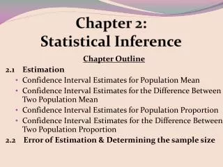
6.2 Confidence Intervals for Means • Size n sample with unknown meanμbut known Var. 2 If X1, …, Xn ~ N(, 2), then Then, confidence interval of is
If we do not know the distribution of X, then when n is large, we Still approximately have (C.L.T.) 2. Size n samplewith unknown mean and Var. 2 Please look Example 1 on P270. ∴ 2 can be replaced by nS2/(n 1). We have an approximate Confidence interval for . (when n is large)
As a matter of fact, if X1,…,Xn~N(, 2), (i.i.d), then X and S2 are independent, and Let’s look Example 2 and 3 on p270-271. Note:SupposeX1,…, Xn~(i.i.d) f(x; ), a r. v. Q(X1,…,Xn; ) is a pivotal quantity (orpivot) if the distribution of Q is independent of all parameters. The above method to find the c. i. is called pivotal inference. As we known, when X1,…,Xn~(i.i.d)N(, 2), is unknown, then is a pivot. Similarly, is also a pivot.
If Y~ b(n, p), we can use the relative frequency Y/n to estimate p. What is the accuracy. 3. The Confidence interval of p =P(success) approximately That is
We have an approximate (100)% c. i. [p1, p2] for p. Replacing p by Y/n in p(1p)/n, we have (P254 Example 1.) for brevity. ∴ we get a c. i.
6.3 Confidence Intervals for Differences of Means 1. C. I. for differences of means of double normal Distributions
The c. i. of 12 can be found from the inequality as follows. The c. i. of 12 can be found from the inequality as follows. Where Swis the mixed samples variance. You can look example 1. on page 278 of the book.
2. The Confidence Intervals for p1 – p2 If Y1~b(n1, p1), Y2 ~ b(n2, p2) and they are independent, Then, the pivot approximately, n1, n2 are large. Again replacing pi by Yi/ni in pi(1 pi)/ni, I =1, 2, we have an approximate (100)% c.i. for p1 p2 as follows : You can look example 2. on page 279 of the book.
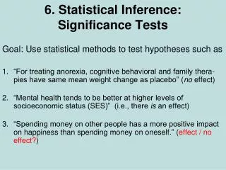
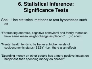
6.4 Tests of Statistical Hypothesis Point estimation and confidence intervals are useful statistical inference procedures. Another type of inference that is frequently used concerns tests of hypotheses. Suppose a r. v. X~f(x; ) where , and =01, 01=. We label hypotheses as H0: 0 versus H1: 1. (6.4.1) The hypothesis H0 is referred to as the null hypothesis while H1 is referred to as the alternative hypothesis. Often the null hypothesis represents no change or no difference from the past while the alternative represents change or difference. The alternative is often referred to as the research worker’s hypothesis.
Example 6.4.1 (Zea Mays Data). In 1878 Charles Darwin recorded some data on the heights of zea mays plants to determine what effect cross-fertilized or self-fertilized had on the heights of zea mays. We will represent the data as (X1, Y1), …, (X15, Y15), where Xi and Yi are the heights of the cross-fertilized and self-fertilized plants, respectively, in the ith pot. Let Wi=XiYi. =E(Wi), our hypotheses are: H0: =0 versus H1: >0. (6.4.2) Hence, 0={0} represents no difference in the treatments and 1=(0, ) represents a difference in the treatments. The decision rule to take H0 or H1 is based on a sample X1, …, Xnfrom the distribution of X and hence, the decision could be wrong.
Table 6.4.1: 22 decision Table for a Test of Hypothesis A test of H0 versus H1 is based on a subset C of D. This set C is called the critical region and its corresponding decision rule (test) is: Reject H0, (Accept H1), if (X1, …, Xn)C Retain H0, (Reject H1), if (X1, …, Xn)Cc. (6.4.3) A Type I error occurs if H0 is rejected when it is true while a Type II error occurs if H0 accepted when H1 is true.
Def. 6.4.1.We say a critical region C is of size if (6.4.4) When 1, we want to maximize 1P[Type II Error]= P[(X1, …, Xn)C]. The probability on the right side of this equation is called the power of the test at . It is the probability that the test detects the alternative when 1 is the true parameter. So minimizing the probability of Type II error is equivalent to maximizing power. We define the power function of a critical region to be C()= P[(X1, …, Xn)C]; 1. (6.4.5) Hence, given two critical regions C1 and C2 which are both of size , C1 is better than C2 if C1() C2() for 1.
Example 6.4.2(Test for a Binomial Proportion of Success). Let X be a Bernoulli r. v. with probability of success p. suppose we want to test at size , H0: p=p0 versus H1: p < p0, (6.4.6) where p0 is specified. As an illustration, suppose “success” is dying from a certain disease and p0 is the probability of dying with some standard treatment. Remark 6.4.1 (Nomenclature). If a hypothesis completely specifies the underlying distribution, such as H0: p=p0, in Example 6.4.2, it is called a simple hypothesis. Most hypotheses, such as H1: p < p0, are composite hypotheses, because they are composed of many simple hypotheses and hence do not completely specify the distribution.
Frequently, is also called the significance level of the test associated with the critical region, and so on. Example 6.4.3(Large Sample Test for the Mean).Let X be a r, v, with mean and finite variance 2. We want to test the hypotheses H0: = 0 versus H1: < 0, (6.4.6) where 0 is specified. To illustrate, suppose 0 is the mean level on a standardized test of students who have been taught a course by a standard method of teaching. Suppose it is hoped that a new method which incorporates computers will have a mean level > 0, where =E(X) and X is the score of a student taught by the new method. Example 6.4.4(Test for under Normality).Let X have a N(, 2) distribution. Consider the hypotheses
H0: = 0 versus H1: < 0, (6.4.6) where 0is specified. Assume that the desired size of the test is , for 0< <1. Suppose X1, …, Xn is a r. s. from X. using the distribution of t(n 1), it is easy to show that the following rejection rule has exact level : Reject H0 in favor of H1 if (6.4.7) where t, n1 is the upper critical point of a t distribution with n 1 degrees of freedom; i.e., = P(T > t, n1). This is often called the t test of H0: = 0.
6.5 Additional Comments About Statistical Tests All of the alternative hypotheses considered in section 6.4 were one-sided hypotheses. For illustration, in exercise 6.42 we tested H0: =30,000 against the one-sided alternative H1: >30,000, where is the mean of a normal distribution having standard deviation = 5000. Perhaps in this situation, though, we think the manufacturer’s process has changed nut are unsure of the direction. That is, we are interested in the alter-native H1: 30,000. in this section, we further explore hypotheses testing and we begin with the construction of a test for a two sided alternative involving the mean of a r. v.
Example 1 (Large sample Two-Sided Test for the Mean). Let X be a r. v. with mean and finite variance 2. We want to test H0: =0 versus H1: 0 (6.5.1) where 0 is specified. Let X1, …, Xnbe a r. s. from X. We will use the decision rule Reject H0 in favor of H1 if (6.5.2) where h and k are such that Clearly h <k, hence, we have An intuitive rule is to divide equally between the two terms on the right-side of the above expression; that is, h and k chosen by
(6.5.3) By the CLT and the consistency of S2 to 2, we have under H0 that This and (6.5.3) leads to the approximate decision rule: Reject H0 in favor of H1 if (6.5.4) To approximate the power function of the test, we use the CLT. Upon substituting for S, it readily follows that the approximate power function is (6.5.5)
() is strictly decreasing for <0 and strictly increasing for >0. Where (z) is the pdf of a standard normal r. v. Accept H0if and only if (6.5.6) Example 2.Let X1, …, Xn1 iid from N(1, 2); Y1, …, Yn2 iid from N(2, 2). At =0.05, reject H0 : 1=2 and accept the one-sided alternative H1 : 1>2if where
Example 3.Say X~b(1, p). Consider testing H0: p=p0 against H1: p<p0. Let X1, …, Xn be a r. s. from X and let To test H0 versus H1, we use either If n is large, both Z1 and Z2 have approximate N(0, 1) distributions provided that H0: p=p0 is true. If is given, c can be decided. is a (1 )100% approximate c. i. for p.
Example 4.Let X1, …, X10 be a r. s. from P( ). A critical region for testing H0: =0.1 against H1:>0.1 is given by (p290) Remark (Observed Significance Level). Not many statisticians like randomized tests in practice, because the use of them means that two statisticians could make the same assumptions, observe the same data, apply the same test, and yet make different decisions. Hence they usually adjust their significance level so as not to randomize. As a matter of fact, many statisticians report what are commonly called observed significance level or p-values
6.6 Chi-Square Tests In this section we introduce tests of statistical hypotheses called chi-square tests. A test of this sort was originally proposed by Karl Pearson in 1900, and it provided one of the earlier methods of statistical inference. Let’s now discuss some r. vs. that have approximate chi-square distributions. Let X1 be b(n, p1). Consider the r. v. which has, as n, a limiting distribution of N(0, 1), we strongly suspect that the limiting distribution of Z=Y2 is 2(1).
If Gn(y) represents the cdf of Y, we know that (CLT) Let Hn(z) be the cdf of Z=Y2. Thus, if z 0, (Hn(z)=0, if z < 0) Therefore, the limiting distribution of Y is 2(1). Now, let X1~b(n, p1), X2 = nX1 and p2=1p1.Then X1np1 =(nX2) n(1p2) = (X2np2)
We say, when n is positive integer, that Q1 has a limiting chi-square distribution with 1 degree of freedom. This result can be generalized as follows. Let X1, …, Xk1 have a multinomial distribution with the parameters n and p1, …, pk1. Let Xk = n (X1+…+Xk1) and let pk =1(p1+…+ pk1). Define Qk1 by
It is proved in a more advanced course that, as n, Qk1 has a limiting distribution that is 2(k1). If we accepted this fact, we can say Qk1 has an approximate chi-square distribution with k1 degree of freedom when n is a positive integer. This approximation is good when n is large enough (n 30) and npi 5. The r. v. Qk1may serve as basis of the tests of certain statistical hypotheses which we now discuss. Let the sample space A=A1… Ak, and AiAj=, ij. Let P(Ai) = pi, i = 1, …, k, where pk =1(p1+…+pk1), so that pi is the probability that the outcome of the random experiment of the set Ai. The random experiment is to be repeated n independent times and X will represent the number of times the outcome an element of the set Ai. That is, X1, …, Xk1, Xk=n(X1+…+Xk1) is the multinomial pdf with parameters n, p1, …, pk1.
Consider the simple hypothesis (concerning this multinomial pmf) H0: p1=p10, …, pk1=pk1,0, (pk= pk0 =1p10 …pk1,0), where p10 , …,pk1,0 are specified numbers. It is desired to test H0 against all alternatives. If the hypothesis H0 is true, the r. v. has an approximate 2(k 1) distribution. If significance level is given, then the critical region is Qk1 2(k 1). That is P(Qk1 2(k 1))= . This is frequently called a goodness of fit test. There are some illustrative examples as follows. P280~284 Example 1.~4. P296-299