Download

1 / 45
460 likes | 616 Views
Matrix Representations of Graphs. Benjamin Martin, Christopher Mueller, Joseph Cottam, and Andrew Lumsdaine Open Systems Lab/Indiana University. Introduction. Introduction to Visual Similarity Matrices Interpreting Visual Similarity Matrices

E N D
Matrix Representations of Graphs Benjamin Martin, Christopher Mueller, Joseph Cottam, and Andrew Lumsdaine Open Systems Lab/Indiana University
Introduction • Introduction to Visual Similarity Matrices • Interpreting Visual Similarity Matrices • Christopher Mueller, Benjamin Martin, and Andrew Lumsdaine. Interpreting Large Visual Similarity Matrices. In Asia-Pacific Symposium on Visualization, February 2007 • A Comparison of Ordering Algorithms • Christopher Mueller, Benjamin Martin, and Andrew Lumsdaine. A Comparison of Vertex Ordering Algorithms for Large Graph Visualization. In Asia-Pacific Symposium on Visualization, February 2007 • BFS Case Study
Visual Similarity Matrices Essentially, draw the adjacency matrix • Axes are labeled with the vertex names • Matrix dots represent graph edges
Visual Similarity Matrices Advantages: • Capable of representing much larger graphs • No risk of occlusion or edge crossings • Good for large and dense graphs, for most tasks See M. Ghoniem, J.-D. Fekete, and P. Castagliola. “On the readability of graphs using node-link and matrix-based representations: a controlled experiment and statistical analysis.” In Information Visualization, volume 4, pages 114–135, 2005.
Visual Similarity Matrices But VSMs must be ordered Expert Ordering NCI AIDs Screen Data Random Ordering So how do we do that?
Questions • How do we order a VSM? • How do we decide between different methods? • How do we interpret the results?
Interpreting VSMs Some features of VSMs are dependent on the matrix ordering, some are not
Interpreting VSMs Straight horizontal or vertical lines show “star” connectivity patterns in a graph. Noncontiguous lines carry the same information as contiguous lines Diagonal lines carry information if they are more than one pixel wide. May have to look at information elsewhere in the matrix… New edges
Interpreting VSMs Wedges appear on the diagonal and represent cliques Off-diagonal blocks are bi-partite sub-graphs. Blank rows or columns for a vertex remove the vertex from the component. Blocks and wedges can be joined across rows and columns: • - A is a clique (mirrored on the diagonal) • - B, C, D are bi-partite sub-graphs • - A + B, A + C are cliques • A + B + C + D is a clique • A and D are independent w/o additional • supporting structures
Interpreting VSMs Some ordering algorithms may produce characteristic patterns in the VSM Envelope footprints are indicative of breadth-first search algorithms. Horizon footprints suggest depth-first algorithms. Galaxy footprints are caused by algorithms that don’t follow direct paths through the graph.
Ordering • Algorithms • Breadth first search • Depth first search • Degree ordering • Reverse Cuthill-McKee (RCM) • King’s algorithm • Sloan’s algorithm • Separator tree • Spectral Ordering
Data • Synthetic Graphs (100, 500, 1000 vertices) • Erdős-Renyi • Small World • Power-law • K-partite • “K-linear-partite” • Real • COGSimilar - 1770 vertices, 290k edges • COGDissimilar - 2030 vertices, 158k edges • NCIca - 436 vertices, 18.6k edges • NCIall - 42,750 vertices, 3.29M edges
Methods: VSM Preparation … (1) (2) (3) (4) Create or load each graph Create two initial vertex orderings in memory: original and random Apply each algorithm to each initial ordering Generate hi-res (1000x1000) and lo-res (100x100) version of each VSM
Coarse/fine structure Coarse structure Minimal structure No structure Stable: similar structure Structure: dissimilar structure Ordered: only original has structure No structure Methods: Evaluation Stability: Compare original and random pairs with new ordering Interpretability: Evaluate quality of structure in each image
Results: Stability • Synthetic graphs tended to be stable for all algorithms • Real graphs • “Stable” for degree, partitioning, and spectral algorithms • “Structured” for search-based algorithms Stability is dependent on the graph and algorithm
Results: Interpretability Graphs with regular or dense connection patterns exhibited coarse and fine structure Structural artifacts from each algorithm were evident across all graph types
Results: BFS • “Envelope” footprint • Retains some internal structure from original ordering • Imparts structure on ER graphs
Results: DFS • “Horizon” footprints • Strong diagonal • Some internal structure added to visualization
Results: Degree • Visually reveals degree distribution • Poorest overall results
Results: RCM and King • Both impart additional structure within the envelope created by the BFS
Results: Separator Tree • Characterized by a “fat” diagonal • Nearly reproduces ordering for small world graph
Results: Sloan • Best overall • Similar results, regardless of initial ordering, for all graph types
Results: Spectral • “Galaxy” footprint • Performed well on structured graphs and fully resolved KL5 graphs
Ordering Conclusions • If structure is present in the data, all algorithms provide clues to it • Amount of connectedness has the largest positive impact on ordering quality • Randomness in data has the largest negative impact on ordering quality • Algorithms that looked at global and local properties performed best
Implementation Issues Interactivity is essential for exploring large graphs. Alternate orderings allow for different views and interpretations. Linked views, especially for vertex properties, help explore structural features. Edges (dots) can be colored by weight or category. Anti-aliasing is essential for large, sparse graphs: The graph on the right is easily interpreted as a dense graph with little structure. The image on the left provides a more accurate rendering of the graph.
Some Lessons • VSMs are compelling tools for exploring large graphs • Care must be taken to ensure proper interpretations are made • Interactive tools that provide multiple views of the graph are useful for exploring large VSMs
BFS Case Study BFS shows remarkable consistency over several graph types, especially SWGs Can we better characterize its behavior? Specifically, can we quantify some of the things we’re seeing?
Visual Parameters • Bandwidth and average envelope width • Envelope jump • Envelope terminal • Number of envelope gaps • Average gap width
Graph Measurements • Diameter • Characteristic path length • Global efficiency • Clustering coefficient • Model parameters n, k, p
BFS Case Study We begin by considering fixed n and k, and looking at diameter and average envelope width.
Generalizing What about other n and k?
Summary • Average envelope width is an effective and simple predictor of global efficiency for Watts-Strogatz graphs • Which indirectly gives us the diameter • And hopefully this works with other graph types
Possible directions • Look at more diverse data • Look at other orderings, especially spectral
Acknowledgements Funding: Lily Endowment National Science Foundation grant EIA-0202048. Software and Algorithms: Doug Gregor (Boost Graph Library) Jeremiah Willcock (Separator Tree) Data: Sun Kim (PLATCOM) David Wild (NCI)