Download
1 / 31
310 likes | 450 Views
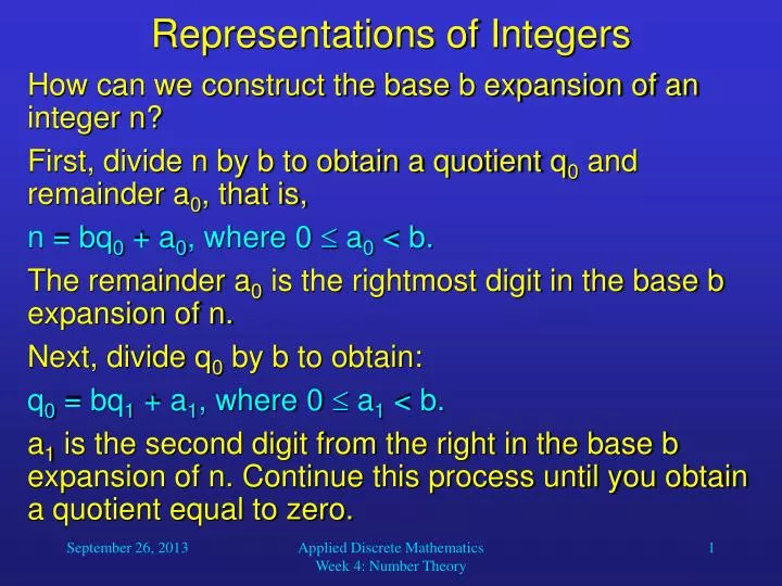
Representations of Integers. How can we construct the base b expansion of an integer n? First, divide n by b to obtain a quotient q 0 and remainder a 0 , that is, n = bq 0 + a 0 , where 0 a 0 < b. The remainder a 0 is the rightmost digit in the base b expansion of n.

E N D
Representations of Integers • How can we construct the base b expansion of an integer n? • First, divide n by b to obtain a quotient q0 and remainder a0, that is, • n = bq0 + a0, where 0 a0 < b. • The remainder a0 is the rightmost digit in the base b expansion of n. • Next, divide q0 by b to obtain: • q0 = bq1 + a1, where 0 a1 < b. • a1 is the second digit from the right in the base b expansion of n. Continue this process until you obtain a quotient equal to zero. Applied Discrete Mathematics Week 4: Number Theory
Representations of Integers • Example:What is the base 8 expansion of (12345)10 ? • First, divide 12345 by 8: • 12345 = 81543 + 1 • 1543 = 8192 + 7 • 192 = 824 + 0 • 24 = 83 + 0 • 3 = 80 + 3 • The result is: (12345)10 = (30071)8. Applied Discrete Mathematics Week 4: Number Theory
Representations of Integers • procedure base_b_expansion(n, b: positive integers) • q := n • k := 0 • while q 0 • begin • ak := q mod b • q := q/b • k := k + 1 • end • {the base b expansion of n is (ak-1 … a1a0)b } Applied Discrete Mathematics Week 4: Number Theory
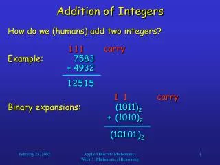
( )2 Addition of Integers carry 1 1 1 • How do we (humans) add two integers? • Example: 7583 + 4932 1 2 5 1 5 carry 1 1 Binary expansions: (1011)2 +(1010)2 1 0 1 0 1 Applied Discrete Mathematics Week 4: Number Theory
Addition of Integers • Let a = (an-1an-2…a1a0)2, b = (bn-1bn-2…b1b0)2. • How can we algorithmically add these two binary numbers? • First, add their rightmost bits: • a0 + b0 = c02 + s0, • where s0 is the rightmost bit in the binary expansion of a + b, and c0 is the carry. • Then, add the next pair of bits and the carry: • a1 + b1 + c0 = c12 + s1, • where s1 is the next bit in the binary expansion of a + b, and c1 is the carry. Applied Discrete Mathematics Week 4: Number Theory
Addition of Integers • Continue this process until you obtain cn-1. • The leading bit of the sum is sn = cn-1. • The result is: • a + b = (snsn-1…s1s0)2 Applied Discrete Mathematics Week 4: Number Theory
Addition of Integers • Example: • Add a = (1110)2 and b = (1011)2. • a0 + b0 = 0 + 1 = 02 + 1, so that c0 = 0 and s0 = 1. • a1 + b1 + c0 = 1 + 1 + 0 = 12 + 0, so c1 = 1 and s1 = 0. • a2 + b2 + c1 = 1 + 0 + 1 = 12 + 0, so c2 = 1 and s2 = 0. • a3 + b3 + c2 = 1 + 1 + 1 = 12 + 1, so c3 = 1 and s3 = 1. • s4 = c3 = 1. • Therefore, s = a + b = (11001)2. Applied Discrete Mathematics Week 4: Number Theory
Addition of Integers • procedure add(a, b: positive integers) • c := 0 • for j := 0 to n-1 {larger integer (a or b) has n digits} • begin • d := (aj + bj + c)/2 • sj := aj + bj + c – 2d • c := d • end • sn := c • {the binary expansion of the sum is (snsn-1…s1s0)2} Applied Discrete Mathematics Week 4: Number Theory
Matrices • A matrix is a rectangular array of numbers. • A matrix with m rows and n columns is called anmn matrix. • Example: is a 32 matrix. A matrix with the same number of rows and columns is called square. Two matrices are equal if they have the same number of rows and columns and the corresponding entries in every position are equal. Applied Discrete Mathematics Week 4: Number Theory
Matrices • A general description of an mn matrix A = [aij]: j-th column of A i-th row of A Applied Discrete Mathematics Week 4: Number Theory
Matrix Addition • Let A = [aij] and B = [bij] be mn matrices. • The sum of A and B, denoted by A+B, is the mnmatrix that has aij + bij as its (i, j)th element. • In other words, A+B = [aij + bij]. • Example: Applied Discrete Mathematics Week 4: Number Theory
Matrix Multiplication • Let A be an mk matrix and B be a kn matrix. • The product of A and B, denoted by AB, is the mnmatrix with (i, j)th entry equal to the sum of the products of the corresponding elements from the i-th row of A and the j-th column of B. • In other words, if AB = [cij], then Applied Discrete Mathematics Week 4: Number Theory
Matrix Multiplication • A more intuitive description of calculating C = AB: - Take the first column of B • Turn it counterclockwise by 90 and superimpose it on the first row of A • Multiply corresponding entries in A and B and add the products: 32 + 00 + 13 = 9 • Enter the result in the upper-left corner of C Applied Discrete Mathematics Week 4: Number Theory
Matrix Multiplication • Now superimpose the first column of B on the second, third, …, m-th row of A to obtain the entries in the first column of C (same order). • Then repeat this procedure with the second, third, …, n-th column of B, to obtain to obtain the remaining columns in C (same order). • After completing this algorithm, the new matrix C contains the product AB. Applied Discrete Mathematics Week 4: Number Theory
Matrix Multiplication • Let us calculate the complete matrix C: 9 7 8 15 15 20 -2 -2 Applied Discrete Mathematics Week 4: Number Theory
Identity Matrices • The identity matrix of order n is the nn matrix In = [ij], where ij = 1 if i = j and ij = 0 if i j: Multiplying an mn matrix A by an identity matrix of appropriate size does not change this matrix: AIn = ImA = A Applied Discrete Mathematics Week 4: Number Theory
Powers and Transposes of Matrices • The power function can be defined for square matrices. If A is an nn matrix, we have: • A0 = In, • Ar = AAA…A (r times the letter A) • The transpose of an mn matrix A = [aij], denoted by At, is the nm matrix obtained by interchanging the rows and columns of A. • In other words, if At = [bij], then bij = aji for i = 1, 2, …, n and j = 1, 2, …, m. Applied Discrete Mathematics Week 4: Number Theory
Powers and Transposes of Matrices • Example: A square matrix A is called symmetric if A = At. Thus A = [aij] is symmetric if aij= aji for alli = 1, 2, …, n and j = 1, 2, …, n. A is symmetric, B is not. Applied Discrete Mathematics Week 4: Number Theory
Zero-One Matrices • A matrix with entries that are either 0 or 1 is called a zero-one matrix. Zero-one matrices are often used like a “table” to represent discrete structures. • We can define Boolean operations on the entries in zero-one matrices: Applied Discrete Mathematics Week 4: Number Theory
Zero-One Matrices • Let A = [aij] and B = [bij] be mn zero-one matrices. • Then the join of A and B is the zero-one matrix with (i, j)th entry aij bij. The join of A and B is denoted by A B. • The meet of A and B is the zero-one matrix with (i, j)th entry aij bij. The meet of A and B is denoted by A B. Applied Discrete Mathematics Week 4: Number Theory
Zero-One Matrices • Example: Join: Meet: Applied Discrete Mathematics Week 4: Number Theory
Zero-One Matrices • Let A = [aij] be an mk zero-one matrix and B = [bij] be a kn zero-one matrix. • Then the Boolean product of A and B, denoted by AB, is the mn matrix with (i, j)th entry [cij], where • cij = (ai1 b1j) (ai2 b2i) … (aik bkj). • Note that the actual Boolean product symbol has a dot in its center. • Basically, Boolean multiplication works like the multiplication of matrices, but with computing instead of the product and instead of the sum. Applied Discrete Mathematics Week 4: Number Theory
Zero-One Matrices • Example: Applied Discrete Mathematics Week 4: Number Theory
Zero-One Matrices • Let A be a square zero-one matrix and r be a positive integer. • The r-th Boolean power of A is the Boolean product of r factors of A. The r-th Boolean power of A is denoted by A[r]. • A[0] = In, • A[r] = AA…A (r times the letter A) Applied Discrete Mathematics Week 4: Number Theory
Let’s proceed to… • Mathematical Reasoning Applied Discrete Mathematics Week 4: Number Theory
Mathematical Reasoning • We need mathematical reasoning to • determine whether a mathematical argument is correct or incorrect and • construct mathematical arguments. • Mathematical reasoning is not only important for conducting proofs and program verification, but also for artificial intelligence systems (drawing inferences). Applied Discrete Mathematics Week 4: Number Theory
Terminology • An axiom is a basic assumption about mathematical structures that needs no proof. • We can use a proof to demonstrate that a particular statement is true. A proof consists of a sequence of statements that form an argument. • The steps that connect the statements in such a sequence are the rules of inference. • Cases of incorrect reasoning are called fallacies. • A theorem is a statement that can be shown to be true. Applied Discrete Mathematics Week 4: Number Theory
Terminology • A lemma is a simple theorem used as an intermediate result in the proof of another theorem. • A corollary is a proposition that follows directly from a theorem that has been proved. • A conjecture is a statement whose truth value is unknown. Once it is proven, it becomes a theorem. Applied Discrete Mathematics Week 4: Number Theory
Rules of Inference • Rules of inference provide the justification of the steps used in a proof. • One important rule is called modus ponens or the law of detachment. It is based on the tautology (p(pq)) q. We write it in the following way: • p • p q • ____ • q The two hypotheses p and p q are written in a column, and the conclusionbelow a bar, where means “therefore”. Applied Discrete Mathematics Week 4: Number Theory
Rules of Inference • The general form of a rule of inference is: • p1 • p2 • . • . • . • pn • ____ • q The rule states that if p1and p2and … and pn are all true, then q is true as well. These rules of inference can be used in any mathematical argument and do not require any proof. Applied Discrete Mathematics Week 4: Number Theory
Rules of Inference q pq _____ p Modus tollens Addition • p • _____ • pq pq qr _____ pr pq _____ p Hypothetical syllogism Simplification p q _____ pq pq p _____ q Conjunction Disjunctive syllogism Applied Discrete Mathematics Week 4: Number Theory