Download
1 / 67
800 likes | 913 Views
Chapter 4. Solving Linear Programming Problems: The Simplex Method. 4.1 The Essence of the Simplex Method. Algebraic procedure Underlying concepts are geometric Revisit Wyndor example Figure 4.1 shows constraint boundary lines Points of intersection are corner-point solutions

E N D
Chapter 4 Solving Linear Programming Problems: The Simplex Method
4.1 The Essence of the Simplex Method • Algebraic procedure • Underlying concepts are geometric • Revisit Wyndor example • Figure 4.1 shows constraint boundary lines • Points of intersection are corner-point solutions • Five points on corners of feasible region are CPF solutions • Adjacent CPF solutions • Share a constraint boundary
The Essence of the Simplex Method In general, for n decision variables, each corner point solution lies at the intersection of n constraint boundaries, and two CPF solutions are adjacent to each other if they share n – 1 constraint boundaries and they are connected by a line segment.
The Essence of the Simplex Method • Optimality test • If a CPF solution has no adjacent CPF solution that is better (as measured by Z, i.e. only checks if any of the edges emanating from the current CPF gives a positive rate of improvement in Z): • It must be an optimal solution
The Essence of the Simplex Method • General procedure with the simplex method - Choose an initial CPF solution such as (0,0) and decide if it is optimal using the optimality test. If yes, stop. Otherwise, iterate until an optimal solution is found. - Move to a better adjacent CPF solution (choose an adjacent CPF solution on the edge where the rate of improvement in Z is positive and largest; there is no need to solve for each adjacent CPF solution, only compare the rate of improvement in Z. After it’s identified, then solve for it and it becomes the current CPF solution and perform the optimality test on it. ) - Iterate until an optimal solution is found
4.2 Setting Up the Simplex Method • First step: convert functional inequality constraints into equality constraints • Done by introducing slack variables • Resulting form known as augmented form • Example: constraint is equivalent to
Setting Up the Simplex Method • Augmented solution • Solution for the original decision variables augmented by the slack variables • Basic solution • Augmented corner-point solution • Basic feasible (BF) solution • Augmented CPF solution
Setting Up the Simplex Method • Properties of a basic solution • Each variable designated basic or nonbasic • Number of basic variables equals number of functional constraints • The nonbasic variables are set equal to zero • Values of basic variables obtained as simultaneous solution of system of equations • If basic variables satisfy nonnegativity constraints, basic solution is a BF solution
Setting Up the Simplex Method • A slack variable in a basic solution equaling 0 indicates this solution lies on the corresponding constraint boundary; if the slack variable is greater than 0, then the basic solution lies on the feasible side of that constraint boundary; if it’s less than 0, then the basic solution lies on the infeasible side of that constraint boundary, so the basic solution is infeasible.
Setting Up the Simplex Method • After three slack variables are introduced, the prototype example has 5 variables and three equations. The number of basic variables is 3 (equals the number of functional constraints) and the number of non-basic variables is 2. The simplex method sets the two non-basic variables to zero, thus each basic solution contains two 0s. For example, let x3 = x4 = 0, the basic solution is (4, 6, 0, 0, -6) which is infeasible. Let x1 = x4 = 0, then (0, 6, 4, 0, 6) is a BF solution. Let x1 = x2 = 0, then (0, 0, 4, 12, 18) is also a BF solution. • Two BF solutions are adjacent if all but one of their non-basic variables are the same. For example, (0, 0, 4, 12, 18) and (0, 6, 4, 0, 6) are adjacent. • The objective function should be written as Z – 3x1 – 5x2 = 0. • The RHS of each functional constraint should be non-negative.
4.3 The Algebra of the Simplex Method • Review row operations and Gaussian elimination method (more detailed review of matrices and matrices operations can be found in Appendix 4 on pages 962 – 966) • Use TI 89 for row operations • Row operations are essential to find the new CPF solution (if there’s any) in each iteration (since the new CPF solution is obtained by solving a system of linear equations for basic variables. Note that the non-basic variables are equal to 0 and the number of equations equals the number of basic variables or the number of functional constraints).
4.4 The Simplex Method in Tabular Form • Tabular form • Records only the essential information: • Coefficients of the variables • Constants on the right-hand sides of the equations • The basic variable appearing in each equation • Example shown in Table 4.3 on next slide
The Simplex Method in Tabular Form • Summary of the simplex method • Initialization • Introduce slack variables (let decision variables be non-basic and slack variables be basic variables initially); note that coefficients for basic variables in row 0 are 0s. • Optimality test • Optimal if and only if every coefficient in row 0 is nonnegative • Iterate (if necessary) to obtain the next BF solution • Determine the entering variable (negative with largest absolute value in row 0) • Determine the leaving basic variables (minimum ratio test; only consider the positive coefficients in the pivot column); renew the record for the basic variables by replacing leaving with entering • Find the new BF solution (perform row operations such that the pivot number is 1 and the other numbers including the number in row 0 in the same column as the pivot number are 0s)
4.5 Tie Breaking in the Simplex Method • Tie for the entering basic variable - This happens there are two or more non-basic variables having the same most negative coefficient in row 0 - Decision may be made arbitrarily, but it can impact the number of iterations to obtain the optimal solution. For example, if we change the prototype example to Z = 3x1 + 3x2, choosing x1 for the entering basic variable results in 3 iterations, choosing x2 results in 2 iterations. • Tie for the leaving basic variable – degeneracy - This happens when performing minimum ratio test, there are two or more minimum ratios. - Choose arbitrarily; the one(s) not chosen will have a value of zero (basic variables having value of zero is called degenerate); it may cause a loop but it rarely happen (if it happens, change the leaving basic variable to another one)
Tie Breaking in the Simplex Method • No leaving basic variable – unbounded Z - This happens when every coefficient in the pivot column is either negative or 0. This implies that Z is unbounded (entering basic can be increased indefinitely without giving negative values to any of the current basic variables) . • This also indicates a mistake has been made to the mathematical model itself.
Tie Breaking in the Simplex Method • Multiple optimal solutions - Simplex method stops after one optimal BF solution is found. • Often other optimal solutions exist and would be meaningful choices. • If in the final tableau when an optimal solution is found, at least one of the non-basic variables having a coefficient of zero in row 0, it indicates that multiple optimal solution exists. • To find other optimal solutions, perform additional iterations by choosing a non-basic variable with a zero coefficient in row 0 as the entering basic variable.
4.6 Adapting to Other Model Forms • Simplex method adjustments • Needed when problem is not in standard form (i.e. maximize Z, ≤ functional constraints, RHS ≥ 0, and all decision variables ≥ 0) • Made during initialization step • Types of non-standard forms - Equal constraints - Negative right-hand side - Functional constraints in ≥ form - Minimizing Z
Adapting to Other Model Forms • Equal constraints: intruding artificial-variable technique - With an equal constraint, there’s no obvious initial BF solution. • A nonnegative artificial (or dummy) variable should be introduced for each equal constraint as if it were a slack variable • Becomes initial basic variable for that equation • Include it in the objective function by multiplying it by a big number - M (as a penalty to have a value > 0) assuming maximizing Z. This is called the Big M method. This method may cause numerical instability. The Two-Phase method (introduced later) is used more often.
Adapting to Other Model Forms II. Minimizing problem Minimizing Z is equivalent to maximizing –Z. III. Negative right hand side Multiply both sides of the constraint by -1 (as a result, ≥ becomes ≤ and ≤ becomes ≥) IV. Functional constraints in ≥ form Introduce surplus variable and then an artificial variable (since after the surplus variable is introduced, the constraint is equivalent to an equation with “=“ sign). For example, the third constraint in the radiation therapy example,
Adapting to Other Model Forms • Solving the radiation therapy problem using the big M method:
Adapting to Other Model Forms Row 0 is not in the proper form for the simplex method (the coefficients of basic variables should be 0; the two artificial variables in this example)
Adapting to Other Model Forms • Using the Two-Phase method (no big M needed) for the Radiation Therapy example Phase 1: all artificial variables are driven to 0 (and since the objective function is Min Z = summation of all artificial variables, so Z is also 0 at the end of phase I) in order to reach an initial BF solution. Use this initial BF solution at the start of phase II. Phase II: all artificial variables are kept at 0 (can be dropped) and perform the Simplex Method which leads to the optimal solution (using the objective function from the real problem). .
Adapting to Other Model Forms • No feasible solutions • Constructing an artificial feasible solution may lead to a false optimal solution • Artificial-variable technique provides a way to indicate whether this is the case: if at least one artificial variable in the final solution using Big M method or Two-Phase method is greater than 0, this implies that the original problem has no feasible solution. The artificial variables should always have values of 0. • Variables are allowed to be negative • Example: negative value indicates a decrease in production rate • Negative values may have a bound or no bound 1. Variable with a bound on negative values allowed
Adapting to Other Model Forms For example, in the prototype example, one of the nonnegativity constraint is changed as follows:
Adapting to Other Model Forms 2. Variables with no bound on the negative values allowed
Adapting to Other Model Forms If more than one decision variable lack lower-bound constraints, to avoid increasing too many variables, the approach can be modified slightly so the number of variables is increased by only one. Replacing each xj that lacks lower-bound constraint as follows:
4.7 Postoptimality Analysis • Simplex method role
Postoptimality Analysis • Reoptimization • Alternative to solving the problem again with small changes • Involves deducing how changes in the model get carried along to the final simplex tableau • Optimal solution for the revised model: • Will be much closer to the prior optimal solution than to an initial BF solution constructed the usual way (and in fact, the prior optimal solution can be used as the initial basic solution for solving the revised model if it’s still feasible and if it’s not feasible, apply the dual simplex method described in Section 8.1), therefore, only a few iterations should be required to re-optimize instead of hundreds or thousands that may be required from an initial BF solution.