Download
1 / 39
390 likes | 505 Views
Wireless Distributed Sensor Challenge Problem: Demo of Physical Modelling Approach. Bart Selman, Carla Gomes, Scott Kirkpatrick , Ramon Bejar, Bhaskar Krishnamachari, Johannes Schneider Intelligent Information Systems Institute, Cornell University & Hebrew University

E N D
Wireless Distributed Sensor Challenge Problem: Demo of Physical Modelling Approach Bart Selman, Carla Gomes, Scott Kirkpatrick, Ramon Bejar, Bhaskar Krishnamachari, Johannes Schneider Intelligent Information Systems Institute, Cornell University & Hebrew University Autonomous Negotiating Teams C&D Meeting, June 27, 2002 Vanderbilt University, Nashville TN
Outline • Overview of our approach • Movie conventions • Computational cost (can be small) • Phase diagram • Connections with distributed agents • We demonstrate results of varying amounts of renegotiation • Enhancements and restrictions • Reduce sector changes • Scale to larger sensor arrays
Overview of Approach • We develop heuristics more powerful than greedy, not compromising speed • Goal: • Principled, controlled, hardness-aware systems
IISI, Cornell University ANTs Challenge Problem • Multiple doppler radar sensors track moving targets • Energy limited sensors • Constrained, fallible communications • Distributed computation • Real time requirements
Physical model (and annealing) • Represent acquisition and tracking goals in terms of a system objective function • Define such that each sensor, with info from its 1-hop neighbors, can determine which target to track • “Energy” per target depends on # of sensors tracking
More on annealing • Target Cluster (TC) is >2 1-hop sensors tracking the same target – enough to triangulate and reach a decision on response. • Classic technique – Metropolis method simulates asynchronous sensor decision, thermal annealing allows broader search (with uphill moves) than greedy, under control of annealing schedule.
Moving targets, tracking and acquisition • 100 sensors, t targets (t=5-30) incident on the array, curving at random. Movies of 100 frames for each of several values of (sensors in range)/target and (1-hop neighbors)/sensor. Sensors on a regular lattice, with small irregularities. Between each frame a “bounce,” or partial anneal using only a low temperature, is performed to preserve features of the previous solution as targets move.
Physical Model as Distributed Agents • To compare with agent-based approaches: • Our sensors are independent agents • At each time step, each chooses a target to track, based on the energy function, and informs its neighbors. • At T=0, sensors optimize locally • T>0 is like renegotiation with reduced constraints, except that “uphill moves” may occur at any point in the search, not only when stuck. • As targets move, sensor re-allocation is done using “heat bumps” – low T is restricted renegotiation, higher T allows more extensive search for alternatives.
Moving Targets -- Movies Conventions: • Targets (blue pts) • Target range (green circles) • Sensors (crosses) • Sectors active in a TC are shown • Target Clusters (red lines) • Fraction of targets covered (thermometer)
Introduce reduced connectivity 2.8 ngbrs/sensor 6.16 ngbrs/sensor
Analysis of physical model results • When t targets arrive at once, perfect tracking can take time to be achieved. • Target is considered “tracked” when a TC of 3+ sensors keeps it in view continuously. • We analyze each movie for longest continuous period of coverage of each target, report minimum and average over all targets.
Analyzing the movies • Summary frames: easy case (10 targets) hard case (30 targets) color code: red (1 TC), green (2 TCs), blue (3 TCs), purple (4TCs) , …
Additional summary information: Total time tracked, max continuous time tracked
Results with moving targets Target visibility range and targets/sensor bounds seen:
Movies to show: • Results of pure agent, agents with renegotiation, and “annealing” operating points • CR10 = 4 ngbrs on average • 15 targets incident on the array • Cases: T0, T0.3, T3.0
Results of renegotiation Harder cases see bigger improvement, but effect of small amounts hard to control.
Control of sector assignment • Previous movies allowed sensor to sample all sectors while choosing target. Now we make that choice only at the outset of time step. • Problem is harder. We lose about 8% average coverage, hold same continuous coverage. An intermediate approach is desireable. • Phase boundary (or threshold of dif ficulty) moves in.
Comparing coverage, 10 targets, CR10 Sectors fixed Sectors varying
Comparing coverage, 10 targets, CR10 Varying sectors Fixed sectors
How much can search be speeded up? Conservative setting (100x) uses <10 msec/sensor/time step (850 MHz Pentium) Further 10-100x reductions possible except near phase bndry.
As the problems get bigger… • Physical model effort, in principle, scales linearly, not exponentially, as number of sensors managed grows. • In our model, biggest cost is the communications cost of keeping cluster information (TC’s) current in a well-connected model with few targets present. As the problem gets uglier, this cost decreases because TC’s get smaller! • Example – series of simulations with 400 sensors, 40-120 targets incoming. One movie can be seen at http://www.cs.huji.ac.il/~kirk/darpa/film.gif .
How often must sectors change? Note that varying sectors change less often, and give better solution.
Fraction of sensors covering targets Once targets spread, nearly all sensors contribute.
Fraction of sensors covering targets Fixing sectors reduces available sensors ~12%.
Average # of TCs per target tracked Not wasteful, >1 TC’s helps handoff as targets move.
Average # of sensors tracking a target Excessive coverage of some targets. Can sensors be freed up to improve detection, save power?
Ways to further improve big array performance: • Explore restricted # of sector changes in a time step. • Reallocate sensors from overtracked targets, e.g. by tuning the potential for high densities. • Introduce target-identity memory to reduce need for continuous tracking. Create a derived MRF object, like edge detection in image processing.
IISI, Cornell University Summary • Graph-based physical models capture the ANTs challenge domain • Results on the tradeoffs between: Computation, Communication, Radar range, and Performance are captured in phase diagram. • Techniques handle realistic constraints, fast enough for use in real distributed system.
IISI, Cornell University The End