Download

1 / 21
210 likes | 334 Views
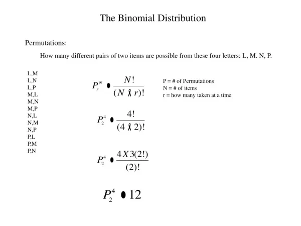
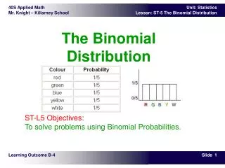
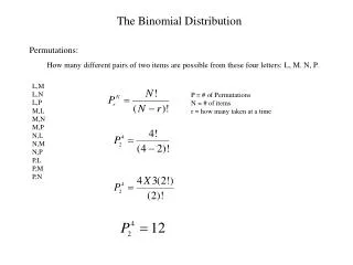
5-3 Additional Properties of The Binomial Distribution. Binomial Experiments. Also called Bernoulli Experiments

E N D
Binomial Experiments Also called Bernoulli Experiments Imagine those boxes of Wheaties again that have pictures of sports stars in them. What if you only want a picture of Tiger Woods? That is, opening a box with Lance or Serena is no good, but Tiger is good?
Binomial Experiments (cont) A Binomial experiment has a fixed number of trials (n) which are independent and repeated under identical conditions. Each trial has only one of two outcomes – Success or Failure The probability of success (p) or failure (q) is the same for every trial The central question will always be: What is the probability of r number of successes out of n trials
Binomial Experiments (cont) Other Binomial (Bernoulli) Trials are - Tossing a coin - Drawing a card (with replacement) - Finding a defective product on an assembly line - Tossing a ring onto bottles at Point Pleasant
Binomial Experiments (cont) How do we find p? Hmmmm… One note: If the selection is made without replacement, is that independent? If the number of trials is small enough with respect to the population, it is considered to be essentially independent, and a Binomial Experiment can be used to approximate the outcome. The value of p will round to be close enough. The book has a good discussion of this.
How does this work? Imagine tossing a coin three times and getting heads exactly two times. How could this happen? Imagine all outcomes HHH, HHT, HTH, HTT, THH, THT, TTH, TTT No heads: 1 One heads: 3 Two heads: 3 Three heads: 1
What if we toss more times? Toss that coin four times HHHH, HHHT, HHTH, HHTT, HTHH, HTHT, HTTH, HTTT THHH, THHT, THTH, THTT, TTHH, TTHT, TTTH, TTTT No heads: 1 One heads: 4 Two heads: 6 Three heads: 4 Four heads: 1 Do those numbers look familiar?
Binomial Experiments (cont) This will look familiar… A binomial experiment is fashioned on a binomial expansion that looks like this:
Binomial Experiments (cont) This will look familiar… A binomial experiment is fashioned on a binomial expansion that looks like this:
Binomial Experiments (cont) From last year you learned how to expand using the shortcuts. The application here is that the formula for a binomial probability from this formula is given by
Binomial Experiments (cont) From last year you learned how to expand using the shortcuts. The application here is that the formula for a binomial probability from this formula is given by p = probability of success; q = failure; r = number of successes in n trials
A few notes… 1. If you are looking for x or fewer (or x or more) successes, you need to compute P(x) + P(x-1) + P(x-2)… That is the probability of tossing 3 or fewer heads = P(3) + P(2) + P(1) + P(0)
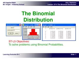
A few notes… 2. Guess what – the calculator can compute binomial probabilities! Hallelujah!! MATH: PRB: 3:nCr Put the n in before you press this button, then press r. Lets try to find 12C2 DISTR: 0: binompdf(n,p,r) gives P(r) DISTR: A: binomcdf(n,p,r) gives P(x ≤ r)
A few notes There is also a table in the back that you should try with one (any one) problem. This table, table 3 in Appendix II has n from 2 to 20 computed probability values for certain p values.
A few notes… 3. μ = np and for a binomial probability model. Remember that μ is also called the expected value
A few notes… 4. The model to decide the number of trials till success is called a Geometric Probability Model for Bernoulli, and the expected value here is
A few notes… 4. The model to decide the number of trials till success is called a Geometric Probability Model for Bernoulli, and the expected value here is
A few notes… 4. The model to decide the number of trials till success is called a Geometric Probability Model for Bernoulli, and the expected value here is The chance of success on the xth trial is
A few notes… 4. The model to decide the number of trials till success is called a Geometric Probability Model for Bernoulli, and the expected value here is The chance of success on the xth trial is Think about last chapter and basic probability… this is based on order mattering
A few notes… 4. Success/Failure condition – A binomial model is described as approximately Normal if np ≥ 10 and np ≥ 10. We’ll discuss that more in the future as well.
Lets try a problem Suppose 20 donors come in for a blood drive. A) If donors line up at random, how many do you expect to examine before you find someone who is a universal donor? Universal donors are O negative. Only about 6% B) what is the probability that the first Universal donor is one of the first four people in line? * C) What is the probability that there are 2 or 3 universal donors? D) What are the mean and standard deviation of the number of universal donors among them? * This means the probability that the first person is plus the probability that the first person is not but the second is, plus the probability that the first and second are not but the third is… - like last chapter