Download
1 / 20
200 likes | 324 Views
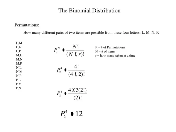
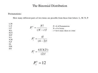
The Binomial Distribution. For the very common case of “Either-Or” experiments with only two possible outcomes. Recognize Binomial Situations. Only two possible outcomes in each trial. Probability for one of the outcomes. Probability for the other outcome.

E N D
The Binomial Distribution For the very common case of “Either-Or” experiments with only two possible outcomes
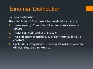
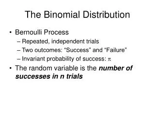
Recognize Binomial Situations • Only two possible outcomes in each trial. • Probability for one of the outcomes. • Probability for the other outcome. • Some definite number of trials, . • They’re independent trials. don’t change. • We’re interested in , probability of a certain count of how many times event happens in those trials.
A special kind of probability distribution • It’s the familiar probability distribution • But only two rows for the two outcomes. • Note that • Because probabilities must always sum to 1.00000 • And this leads to .
The Binomial Probability Formula • Question: If we have trials, what is the probability of occurrences of the “success” event (the one with probability ) • Answer:
Practice with the Formula • Experiment: Roll two dice • Event of interest: “I rolled a 7 or an 11” • Probability of success: (from • Probability of failure: • Number of trials
Practice with the Formula • Find P(2) successes in the seven/eleven game • How about 3 successes?
Sometimes you add probabilities • Probability of at least three wins in five trials • P(X≥3) = P(X=3) + P(X=4) + P(X=5) add them up! • Probability of more than three wins • P(X>3) = P(X=4) + P(X=5) • Probability of at most three wins • P(X≤3) = P(X=0) + P(X=1) + P(X=2) + P(X=3) • Probability of fewer than three wins • P(X<3) = P(X=0) + P(X=1) + P(X=2)
Use the Complement to save time • Example: • “Probability of at least 3 wins” • P(X≥3) = P(X=3) + P(X=4) + … + P(X=49) + P(X=50) • This means 48 calculations and sum results. • EASIER: The complement is “fewer than 3” • Take 1 – [ P(X=0) + P(X=1) + P(X=2) ]
TI-84 Computations • binompdf(n, p, X) = probability of X successes in n trials • Recompute the table and make sure we get the same results as the by-hand calculations. • The “pdf” in “binompdf” stands for “probability distribution function”
TI-84 Computations • binomcdf(n, p, x) = P(X=0) + P(X=1) + … P(X=x) successes in n trials • binomcdf(n, p, x) does lots of little binompdf() for you for x = 0, x = 1, etc. up to the x you told it, and it adds up the results • The “cdf” in “binomcdf” stands for “cumulative distribution function”
binomcdf() and complements • Sevens or elevens, n = 50 trials again • P(no more than 10 successes) • binomcdf(50, 8/36, 10) • P(fewer than 10 successes) • binomcdf(50, 8/36, 9) • P(more than 10 successes) – use complement! • 1 minus binomcdf(50, 8/36, 10) • P(at least 10 successes) – use complement! • 1 minus binomcdf(50, 8/36, 9)
Mean, Variance, and Standard Deviation • We had formulas and methods for probability distributions in general. • The special case of the Binomial Probability Distribution has special shortcut formulas • Mean = • Variance = • Standard deviation =
Mean, Variance, and Standard Deviation • Compute these for the seven-eleven experiment with n = 5 trials • Mean = • Variance = • Standard deviation =
Mean, Variance, and Standard Deviation • Compute these for the seven-eleven experiment with n = 50 trials • Mean = • Variance = • Standard deviation =
Mean, Variance, and Standard Deviation • Compute these for the seven-eleven experiment with n = 100 trials • Mean = and Standard deviation = • “Expected value” – in 100 tosses of two dice, how many seven-elevens are expected? • Remember, the mean of a probability distribution is also called the “expected value”
Standard Deviation • What happens to the standard deviation in the seven-eleven experiment as the number of trials, n, increases?
Advanced TI-84 Exercise • Y1=binompdf(20,8/36,X) • seq(X,X,0,20) STO> L1 • seq(Y1(X),X,0,20) STO> L2 • STAT PLOT for these two lists, histogram • WINDOW Xmin=0, Xmax=20, Ymin=-0.1,Ymax=0.6 • ZOOM 9:ZoomStat