Feature Generation I

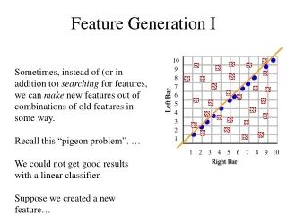
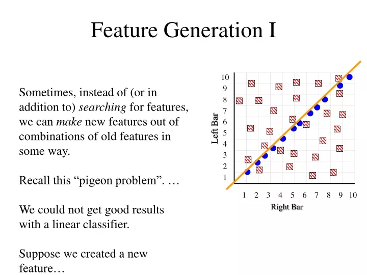
1. 10 9 8 7 6 Left Bar 5 4 3 2 1 1 2 3 4 5 6 7 8 10 9 Right Bar Feature Generation I Sometimes, instead of (or in addition to) searching for features, we can make new features out of combinations of old features in some way. Recall this “pigeon problem”. … We could not get good results with a linear classifier. Suppose we created a new feature…

2. 10 9 8 7 6 Left Bar 5 4 3 2 1 1 2 3 4 5 6 7 8 10 9 Right Bar Feature Generation II Suppose we created a new feature, called Fnew Fnew = |(Right_Bar – Left_Bar)| Now the problem is trivial to solve with a linear classifier. 1 2 3 4 5 6 7 8 10 9 0 Fnew

3. Feature Generation III We actually do feature generation all the time. Consider the problem of classifying underweight, healthy, obese. It is a two dimensional problem, that we can approximately solve with linear classifiers. But we can generate a feature call BMI, Body-Mass Index. BMI = height/ weight2 This converts the problem into as easy 1D problem 18.5 24.9 BMI

4. Let us start with a review/preview Feature generation For many problems, this is the key issue. What if there was a classification algorithm, that could automatically generate higher level features… 1 63

5. What are connectionist neural networks? • Connectionism refers to a computer modeling approach to computation that is loosely based upon the architecture of the brain. • Connectionist approaches are very old (1950’s), but is recent years (under the name Deep Learning) they have become very competitive, due to: • Increases in computational power • Availability of lots of data • Algorithmic insights

6. Neural Network History • History traces back to the 50’s but became popular in the 80’s with work by Rumelhart, Hinton, and Mclelland • A General Framework for Parallel Distributed Processing in Parallel Distributed Processing: Explorations in the Microstructure of Cognition • Peaked in the 90’s, died down, now peaking again: • Hundreds of variants • Less a model of the actual brain than a useful tool, but still some debate • Numerous applications • Handwriting, face, speech recognition • Vehicles that drive themselves • Models of reading, sentence production, dreaming • Debate for philosophers and cognitive scientists • Can human consciousness or cognitive abilities be explained by a connectionist model or does it require the manipulation of symbols?

7. Although heterogeneous, at a low level the brain is composed of neurons • A neuron receives input from other neurons (generally thousands) from its synapses • Inputs are approximately summed • When the input exceeds a threshold the neuron sends an electrical spike that travels that travels from the body, down the axon, to the next neuron(s) The point at which neurons join other neurons is called a synapse

8. Neural Networks • We are born with about 100 to 200 billion neurons • A neuron may connect to as many as 100,000 other neurons • Many neurons die as we progress through life • We continue to learn

9. From a computational point of view, the fundamental processing unit of a brain is a neuron • Moreover, neurons are also the brains unit of memory. • This must be true, since there is really nothing else in the brain.

10. Simplified model of computation • Imagine you have a neuron that has many input dendrites that receive a signal from your cones (cones are the photo receptors in your eye that are sensitive to light intensity). • If only a few send a signal, there is no activation. • When many send a signal, the neuron sends an electrical spike that travels to a muscle, that closes the eyes. • However, note that while some dendrites do receive data from the eyes, ears, nose, heat/pressure from skin etc, and some axons do send signals to muscles. 99.999% of neurons just communicate with other neurons. The story above is too simple, there will be many layers of neurons involved in even blinking

11. 200 billion neurons, 32 trillion synapses Element size: 10-6m Energy use: 25W Processing speed: 100 Hz Parallel, Distributed Fault Tolerant Learns: Yes Intelligent/Conscious: Usually Several billion bytes RAM but trillions of bytes on disk Element size: 10-9 m Energy watt: 30-90W (CPU) Processing speed: 109 Hz Serial, Centralized Generally not Fault Tolerant Learns: Some Intelligent/Conscious: Generally No Comparison of Brains and Traditional Computers

12. The First Neural Networks McCulloch and Pitts produced the first neural network in 1943 Their goal was not classification/AI, but to understand the human brain Many of the principles can still be seen in neural networks of today

13. X1 X3 Y 2 2 X2 -1 The First Neural Networks Consisted of: A set of inputs - (dendrites) A set of resistances/weights – (synapses) A processing element - (neuron) A single output - (axon)

14. X1 X3 Y 2 X2 2 -1 The activation of a neuron is binary. That is, the neuron either fires (activation of one) or does not fire (activation of zero).

15. X1 X3 Y X1 X3 Y 2 2 X2 X2 2 2 -1 -1 For the network shown here the activation function for unit Y is: f(y_in) = 1, if y_in >= θ; elsef(y_in) = 0 where y_in is sum of the total input signal received; θ is the threshold for Y

16. X1 X3 Y 2 X2 2 -1 Neurons in a McCulloch-Pitts network are connected by directed, weighted paths

17. X1 X3 Y 2 X2 2 -1 If the weight on a path is positive the path is excitatory, otherwise it is inhibitory x1 and x2 encourage the neuron to fire x3 prevents the neuron from firing

18. X1 X3 Y 2 X2 2 -1 Each neuron has a fixed threshold. If the total input into the neuron is greater than or equal to the threshold, the neuron fires

19. X1 X3 Y 2 X2 2 -1 It takes one time step for a signal to pass over one connection. One clock cycle.

20. The First Neural Networks Using McCulloch-Pitts model we can model logic functions Let’s look at some examples

21. 1 X1 X2 Y 1 AND Function The AND Function If (X1 * 1) + (X2 * 1) ≥ Threshold(Y) Output 1 Else Output 0 Threshold(Y) = 2

22. 1 1 1 Y 1 AND Function Case 1 The AND Function If (1 * 1) + (1 * 1) ≥ 2 Output 1 Else Output 0 1 Threshold(Y) = 2

23. 1 1 0 Y 1 AND Function Case 2 The AND Function If (1 * 1) + (0 * 1) ≥ 2 Output 1 Else Output 0 0 Threshold(Y) = 2

24. 1 0 1 Y 1 AND Function Case 3 The AND Function If (0 * 1) + (1 * 1) ≥ 2 Output 1 Else Output 0 0 Threshold(Y) = 2

25. 1 0 0 Y 1 AND Function Case 4 The AND Function If (0 * 1) + (0 * 1) ≥ 2 Output 1 Else Output 0 0 Threshold(Y) = 2

26. 2 X1 X2 Y 2 OR Function The OR Function If (X1 * 2) + (X2 * 2) ≥ Threshold(Y) Output 1 Else Output 0 Threshold(Y) = 2

27. X1 X2 Y An AND-NOT function calculates A B The AND NOT Function If (X1 * 2) + (X2 * -1) ≥ Threshold(Y) Output 1 Else Output 0 2 -1 AND NOT Function Threshold(Y) = 2

28. X1 X2 Y Expressiveness of the McCulloch-Pitts Network • Our success with AND, OR and AND-NOT might lead us to think that we can model any logic function with McCulloch-Pitts Networks. • What weights/threshold could we use for XOR? • It is easy to see that this is not possible! • However, there is a trick if we combine several neurons in layers.. ? ? XOR Function

29. XOR X1 X2 Y 1 1 0 Y X1 X2 Z2 1 0 1 0 1 1 0 0 0 We know that we can write XOR as a disjunction of AND-NOTs X1 XOR X2 = (X1 AND NOT X2) OR (X2 AND NOT X1) So we can make a XOR from these atomic parts…. -1 2 2 X1 XOR X2 = (X1 AND NOT X2) OR (X2 AND NOT X1)

30. XOR X1 X2 Y 1 1 0 Z1 Y X1 X2 1 0 1 0 1 1 0 0 0 2 2 -1 X1 XOR X2 = (X1 AND NOT X2) OR (X2 AND NOT X1)

31. XOR X1 X2 Y 1 1 0 Y Z1 Z2 1 0 1 0 1 1 0 0 0 2 2 X1 XOR X2 = (X1 AND NOT X2) OR (X2 AND NOT X1)

32. XOR XOR Function X1 X2 Y 1 1 0 Z2 X2 Y X1 Z1 1 0 1 0 1 1 0 0 0 2 2 -1 -1 2 2 The XOR Function X1 XOR X2 = (X1 AND NOT X2) OR (X2 AND NOT X1)

33. 10 9 8 7 6 5 4 3 B X2 X1 Y 2 1 1 2 3 4 5 6 7 8 9 10 A Linear Function What else can neural nets represent? With a single layer, by carefully setting the weights and the threshold, you can represent any linear function. Note the inputs are now real numbers.

34. 10 9 8 7 6 5 4 3 C G E B Y X8 Y X7 X2 X6 Y X4 Y X1 X3 X5 2 1 1 2 3 4 5 6 7 8 9 10 A F H D What else can neural nets represent? With a multiple layers, by carefully setting the weights and the threshold, you can represent any arbitrary function! Arbitrary Functions

35. 10 9 8 7 6 5 4 3 G B E C X5 Y X7 Y Y X8 X1 Y X3 X2 X4 X6 2 1 1 2 3 4 5 6 7 8 9 10 H D F A What else can neural nets represent? With a multiple layers, by carefully setting the weights and the threshold, you can represent any arbitrary function. Stop! Just because you can represent any function, does not mean you can learn any function. Arbitrary Functions

36. C B G X7 Y X8 Y X1 X4 X3 X2 Y D A H Stop! Just because you can represent any function, does not mean you can learn any function. We make do simple logic functions, and linear classifiers by hand. But suppose I want the input to be a 1,000 by 1,200 image, and the output to be 1|0(cat|dog) Then there are 1,200,000 inputs for the (B/W) image. Even if the weights are binary (and they are not), then there are 21200000 possibilities. Our only hope is somehow learn the weights. • (cat) • (dog)

37. Y X3 -1.2 X1 X2 First, some generalizations.. We allow the inputs to be arbitrary real numbers We allow the weights to be arbitrary real numbers We allow the thresholds to be arbitrary real numbers The first two means that the output could be very large (positive or negative) However, we prefer the output to be bounded between 0 or 1 (or sometimes, -1 to 1), so we can use a sigmoid (or similar) function to “squash” the function into the desired range. A B C -23.4

38. Learning a Neural Network with BackPropagation A dataset Features class 1.4 2.7 1.9 0 3.8 3.4 3.2 0 6.4 2.8 1.7 1 4.1 0.1 0.2 0 etc …

39. Training the neural network Features class 1.4 2.7 1.9 0 3.8 3.4 3.2 0 6.4 2.8 1.7 1 4.1 0.1 0.2 0 etc …

40. Training data Features class 1.4 2.7 1.9 0 3.8 3.4 3.2 0 6.4 2.8 1.7 1 4.1 0.1 0.2 0 etc … Initialise with random weights

41. Training data Features class 1.4 2.7 1.9 0 3.8 3.4 3.2 0 6.4 2.8 1.7 1 4.1 0.1 0.2 0 etc … Present a training pattern 1.4 2.7 1.9

42. Training data Features class 1.4 2.7 1.9 0 3.8 3.4 3.2 0 6.4 2.8 1.7 1 4.1 0.1 0.2 0 etc … Feed it through to get output 1.4 2.7 0.8 1.9

43. Training data Features class 1.4 2.7 1.9 0 3.8 3.4 3.2 0 6.4 2.8 1.7 1 4.1 0.1 0.2 0 etc … Compare with target output 1.4 2.7 0.8 0 1.9 error 0.8

44. Training data Features class 1.4 2.7 1.9 0 3.8 3.4 3.2 0 6.4 2.8 1.7 1 4.1 0.1 0.2 0 etc … Adjust weights based on error 1.4 2.7 0.8 0 1.9 error 0.8

45. Training data Features class 1.4 2.7 1.9 0 3.8 3.4 3.2 0 6.4 2.8 1.7 1 4.1 0.1 0.2 0 etc … Present a training pattern 6.4 2.8 1.7

46. Training data Features class 1.4 2.7 1.9 0 3.8 3.4 3.2 0 6.4 2.8 1.7 1 4.1 0.1 0.2 0 etc … Feed it through to get output 6.4 2.8 0.9 1.7

47. Training data Features class 1.4 2.7 1.9 0 3.8 3.4 3.2 0 6.4 2.8 1.7 1 4.1 0.1 0.2 0 etc … Compare with target output 6.4 2.8 0.9 1 1.7 error -0.1

48. Training data Features class 1.4 2.7 1.9 0 3.8 3.4 3.2 0 6.4 2.8 1.7 1 4.1 0.1 0.2 0 etc … Adjust weights based on error 6.4 2.8 0.9 1 1.7 error -0.1

49. Training data Features class 1.4 2.7 1.9 0 3.8 3.4 3.2 0 6.4 2.8 1.7 1 4.1 0.1 0.2 0 etc … And so on …. 6.4 2.8 0.9 1 1.7 error -0.1 Repeat this thousands, maybe millions of times – each time taking a random training instance, and making slight weight adjustments Algorithms for weight adjustment are designed to make changes that will reduce the error

50. The decision boundary perspective… Initial random weights