Download
1 / 15
150 likes | 152 Views
Explore the various approaches for optimal feature generation, including scatter matrices, Karhunen-Loeve transform, subspace classification, and independent component analysis.

E N D
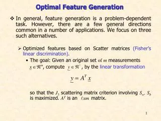
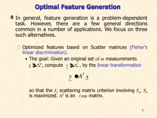
Optimal Feature Generation • In general, feature generation is a problem-dependent task. However, there are a few general directions common in a number of applications. We focus on three such alternatives. • Optimized features based on Scatter matrices (Fisher’s linear discrimination). • The goal: Given an original set of m measurements , compute , by the linear transformation so that the J3 scattering matrix criterion involving Sw, Sb is maximized. AT is an matrix.
The basic steps in the proof: • J3 = trace{Sw-1Sm} • Syw = ATSxwA, Syb = ATSxbA, • J3(A)=trace{(ATSxwA)-1 (ATSxbA)} • Compute Aso that J3(A) is maximum. • The solution: • Let Bbe the matrix that diagonalizes simultaneously matrices Syw, Syb , i.e: BTSywB = I , BTSybB = D where Bis a ℓxℓ matrix and Daℓxℓdiagonal matrix.
Let C=ABanmxℓ matrix. If A maximizes J3(A) then The above is an eigenvalue-eigenvector problem. For an M-class problem, is of rank M-1. • If ℓ=M-1, choose C to consist of the M-1 eigenvectors, corresponding to the non-zero eigenvalues. The above guarantees maximum J3 value. In this case: J3,x = J3,y. • For a two-class problem, this results to the well known Fisher’s linear discriminant For Gaussian classes, this is the optimal Bayesian classifier, with a difference of a threshold value .
If ℓ<M-1, choose the ℓ eigenvectors corresponding to the ℓlargest eigenvectors. • In this case, J3,y<J3,x, that is there is loss of information. • Geometric interpretation. The vector is the projection of onto the subspace spanned by the eigenvectors of .
Principal Components Analysis (The Karhunen – Loève transform): • The goal: Given an original set of m measurements compute for an orthogonalA, so that the elements of are optimally mutually uncorrelated. That is • Sketch of the proof:
If A is chosen so that its columns are the orthogonal eigenvectors of Rx, then where Λis diagonal with elements the respective eigenvalues λi. • Observe that this is a sufficient condition but not necessary. It imposes a specific orthogonal structure on A. • Properties of the solution • Mean Square Error approximation. Due to the orthogonality of A:
Define • The Karhunen – Loève transform minimizes the square error: • The error is: It can be also shown that this is the minimum mean square error compared to any other representation of x by an ℓ-dimensional vector.
In other words, is the projection of into the subspace spanned by the principal ℓ eigenvectors. However, for Pattern Recognition this is not the always the best solution.
Total variance: It is easily seen that Thus Karhunen – Loève transform makes the total variancemaximum. • Assuming to be a zero mean multivariate Gaussian, then the K-L transform maximizes the entropy: of the resulting process.
Subspace Classification. Following the idea of projecting in a subspace, the subspace classification classifies an unknown to the class whose subspace is closer to . The following steps are in order: • For each class, estimate the autocorrelation matrix Ri, and compute the mlargest eigenvalues. Form Ai, by using respective eigenvectors as columns. • Classify to the class ωi, for which the norm of the subspace projection is maximum According to Pythagoras theorem, this corresponds to the subspace to which is closer.
Independent Component Analysis (ICA) In contrast to PCA, where the goal was to produce uncorrelated features, the goal in ICA is to produce statistically independent features. This is a much stronger requirement, involving higher to second order statistics. In this way, one may overcome the problems of PCA, as exposed before. • The goal: Given , compute so that the components of are statistically independent. In order the problem to have a solution, the following assumptions must be valid: • Assume that is indeed generated by a linear combination of independent components
Φis known as the mixing matrix and W as the demixing matrix. • Φmust be invertible or of full column rank. • Identifiability condition:All independent components, y(i), must be non-Gaussian. Thus, in contrast to PCA that can always be performed, ICA is meaningful for non-Gaussian variables. • Under the above assumptions, y(i)’s can be uniquely estimated, within a scalar factor.
Common’s method: Given , and under the previously stated assumptions, the following steps are adopted: • Step 1: Perform PCA on : • Step 2: Compute a unitary matrix, , so that the fourth order cross-cummulants of the transform vector are zero. This is equivalent to searching for an that makes the squares of the auto-cummulants maximum, where, is the 4th order auto-cumulant.
Step 3: • A hierarchy of components: which ℓ to use? In PCA one chooses the principal ones. In ICA one can choose the ones with the least resemblance to the Gaussian pdf.
Example: The principal component is , thus according to PCA one chooses as y the projection of into . According to ICA, one chooses as ythe projection on . This is the least Gaussian. Indeed: K4(y1) = -1.7 K4(y2) = 0.1 Observe that across , the statistics is bimodal. That is, no resemblance to Gaussian.