Download
1 / 16
200 likes | 527 Views
Physics 430: Lecture 9 Curvilinear Systems, Central Forces. Dale E. Gary NJIT Physics Department. O. 4.7 Curvilinear One-Dimensional Systems.

E N D
Physics 430: Lecture 9 Curvilinear Systems, Central Forces Dale E. Gary NJIT Physics Department
O 4.7 Curvilinear One-Dimensional Systems • In addition to an object moving in one dimension in space, such as the horizontal or vertical motions we have been dealing with, we can also treat constrained motion along a curved path in terms of 1 dimension. An example is a bead threaded onto a curved, rigid wire on which it can slide without friction. • Such a curve can be specified in terms of its three-dimensional (x, y, z) coordinates, which might require three separate equations, but we could instead use a single, parametric equation, i.e. specified the bead’s location in terms of a single parameter, say its distance s along the wire from some origin O. With such a choice, problems can be solved as if they were one-dimensional. • The speed (not velocity) is written so the kinetic energy is compared with for a straight track. However, the force is a little more complicated, since the wire exerts a force of constraint. But notice that the constraint force does no work, since it is not in the direction of motion, but only perpen- dicular. We only care about the tangential force Ftang, which is
Potential Energy of Tangential Forces • If all of the tangential forces are due to conservative forces, then we can define a potential energy U(s) such that Ftang = -dU/ds. In this case, the total energy E = T + U is constant, and we can use all of the ideas we have discussed for the one-dimensional case. • In particular, points along s where U(s) is a minimum are stable equilibrium points, and points where U(s) is a maximum are unstable. • There are many problems that at first appear to be more complicated than a bead on a wire, but they are nevertheless one-dimensional and so can be solved using these ideas. • A system composed of many bodies all in motion may seem multi-dimensional, but if they are connected by struts or strings so that the position of the system can be described by a single parameter, then they can be considered one-dimensional. • Let’s take a look at a couple of examples.
C B b h q r O Example 4.7 Stability of a Cube Balanced on a Cylinder • Statement of Problem: • A hard rubber cylinder of radius r is held fixed with its axis horizontal, and a wooden cube of mass m and side 2b is balanced on top of the cylinder, with its center vertically above the cylinder’s axis and four of its sides parallel to the axis. The cube cannot slip on the rubber of the cylinder, but can of course rock from side to side, as shown in the figure. By examining the cube’s potential energy, find out if the equilibrium with the cube centered above the cylinder is stable or unstable. • Solution: • Note that the system is one-dimensional, since its position can be parameterized by a single parameter, q. The constraint forces are the normal and frictional forces of the cylinder on the cube (because the cube does not slide), which do no work (because they are perpendicular to the motion). The only other force is gravity, which is a conservative force, so we can define the potential energy as U = mgh, where h is the height of the CM of the cube above the CM of the cylinder. • If there is any trick, it is to recognize that BC = rq.
q Example 4.7 Stability of a Cube Balanced on a Cylinder • Solution, cont’d: • The angle BC makes from the horizontal is also q. • The length of h is BC sin q + (r+b) cos q = rq sin q + (r+b) cos q. • This let’s us write the potential energy of the system as • Remember that the equilibrium position will be a location where the slope of U is zero (dU/dq = 0), and it will be stable if the curvature is upward (d2U/dq 2 > 0). C B b h q r O • The value of q for which the derivative is zero is found by • This is zero when q = 0, which confirms the obvious—the cube can be balanced directly on top of the cylinder. But is the balance precarious? To find out: • At the equilibrium position q = 0, this is just mg(r -b), which is positive for r > b. Cube must be smaller than cylinder
x FT m1 FT m2 m1g m2g Another Example—Atwood Machine • The Atwood Machine provides another example of a system with several moving parts that can be cast into a one-dimensional framework. • Here the pulley is massless (not essential to the problem) and the cable connecting the two masses cannot stretch. • The position of the whole system can be determined by the position x of the mass below the center of the pulley. • Consider the energies of the two masses after a displacement: where DT1 is the change in kinetic energy after the displacement, DU1 is the change in potential energy due to the displacement, and W1ten is the work done during the displacement against the tension force FT. • The tension force is exactly the same on the two masses, so the work done by tension is equal and opposite, i.e.
x FT m1 FT m2 m1g m2g Another Example—Atwood Machine • Adding the two energies, then, the work done by tension drops out and the total change in energy is zero: • In other words, the total mechanical energy is conserved. • It happens that many systems that contain several particles that are constrained in some way (by strings, struts, or a track) can be treated in this way. • The constraint forces are crucially important for determining how the system moves, but they do no work on the system, so when using energy to solve problems we can simply ignore the constraint forces. • For each particle a, with potential energy Ua, the total energy is constant.
b h q H l - H m M Problem 4.36 • Statement of the problem, part (a): • A metal ball (mass m) with a hole through it is threaded on a frictionless vertical rod. A massless string (length l) attached to the ball runs over a massless, frictionless pulley and supports a block of mass M, as show in the figure. The postions of the two masses can be specified by the one angle q. (a) Write down the potential energy U(q). (The PE is given easily in terms of the heights shown as h and H. Eliminate these two variables in favor of q and the constants b and l. Assume that the pulley and ball have negligible size.) • Solution to part (a): • The PE is just We need to write h and H in terms of l, b, and q, but clearly h = (l - H) cos q, while b =(l - H) sin q. Thus, • Plugging into the expression for U, we have • We are free to drop the uninteresting constant Mgl, which amounts to choosing a different zero for U(q), so
b h q H l - H m M Problem 4.36 • Statement of the problem, part (b): • (b) By differentiating U(q) find whether the system has an equilibrium position, and for what values of m and M equilibrium can occur. Discuss the stability of any equilibrium positions. • Solution to part (b): • Taking the derivative and setting it to zero, we have • Multiplying through by sin2q (note q cannot be zero), and dividing by gb, we have • So equilibria occur at which can only happen when m < M. In that case, there is an equilibrium at • Normally, to see if this is a stable equilibrium, take the second derivative, evaluation at q = qo, and check if it is positive (stable) or negative (unstable). In this case, that leads to a very nasty expression. Instead, imagine pulling the mass m downward (q < qo), letting go, and asking what direction the net force acts. It is clearly upward, tending to restore the equilibrium. Likewise, moving the mass upward leads to a net force downward. Hence the equilibrium is stable.
4.8 Central Forces • We can treat central force problems (such as gravitation and electric force problems) using some of the simplicity provided by one-dimensional problems, because the symmetry of the problems mean that the dependence of the motion can be cast into one involving only the radial component. • Any central force can be written generally as where f(r) gives the magnitude of the force as a function of position r. • Examples are the Coulomb force and the gravitational force • These forces have two properties not necessarily shared by all central forces: 1) they are conservative, and 2) they are spherically symmetric (or rotationally invariant). That is, the magnitude of the force does not depend on the direction of r, but depends only on the magnitude of r, i.e. • What is remarkable is that, for central forces, these two conditions always go together. That is,
r cosq r sinq cos f r sinq sin f r sinq Spherical Polar Coordinates • One way to prove the foregoing statement , we can use spherical polar coordinates. This gives us a good opportunity to introduce them, which we do now. • We already introduced polar coordinates and noted how the r and f unit vectors work. We also extended that to a z component in cylindrical coordinates. In spherical polar coordinates, in contrast, we introduce another angular variable q, called the polar angle (or zenith angle when talking about sky coordinates from some local position on the Earth). The relationships are noted in the figure below. • By inspection of this figure, you should be able to see that • Note that the unit vectors all point in the directions of increase in the vectors. The direction of the unit vector is obvious. The and unit vectors are tangent to the lines of “latitude” and “longitude” through the point. z q r y f x
Circumference 0 Circumference 2pr sin q Circumference 2pr note, not just dq note, not just rdf Gradient in Spherical Polar Coordinates • We would like to express the gradient of a function f in spherical polar coordinates, but before we do, we note that the dot product in these coordinates behaves just as you would expect. If • Then the dot product is • Recall that the gradient of a function f in cartesian coordinates was • Recall also that the change in f due to a small displacement dr is • All we need to do, then, is express the displacement in spherical polar coordinates. z r q y f x dV=dr rdq r sinq df = r2 dr sinq dq df
Gradient in Spherical Polar Coordinates • We can rewrite completely generally as but df is also • Equating these, term by term, we must have • Writing this more compactly, we have • You can see that this is somewhat more complicated than in cartesian coordinates. Likewise the other operators of vector calculus are also more complicated, like the divergence and curl. The expressions for these are shown on the inside back cover of the text.
Conservative and Spherically Symmetric Central Forces • Now we are ready to show that central forces that are conservative are also spherically symmetric, and those that are spherically symmetric are also conservative. • Let’s first assume that the force F(r) is conservative and prove that means it must be spherically symmetric. Because it is conservative, we can express it as the gradient of a scalar potential energy. • Because the force is central, only its radial component can be nonzero, so the last two terms must be zero, i.e. That means the potential energy is spherically symmetric, hence the force is too: • We will show the converse in a moment. The point, though, is that problems involving central forces that are spherically symmetric are nearly as simple as one-dimensional problems, as we will see in Chapter 8.
Problem 4.43 • Statement of the Problem: • In Section 4.8 I claimed that a force F(r) that is central and spherically symmetric is automatically conservative. Here are two ways to prove it: (a) Since F(r) is central and spherically symmetric, it must have the form Using cartesian coordinates, show that this implies that • Solution to part (a): • The first thing we need to do is express in terms of x,y,z coordinates. To do this, recall that • Thus, Taking the curl, we have • To deal with a term like , we use the chain rule and write
Problem 4.43-cont’d • Solution to part (a), cont’d: • You can easily show that the partial derivative and likewise for the other partial derivatives of r. Thus, the first term is • Obviously, the same will be true for the other components, so indeed, • We saw last time that this is enough to ensure that the work done by F is path independent, hence, the force is conservative, which is what we needed to show. • Statement of the problem, part (b): • Even quicker, using the expression given inside the back cover for in spherical polar coordinates, show that • Solution to part (b): • Because the force is central, it has only a radial component fr, hence the expression