Download
1 / 31
310 likes | 398 Views
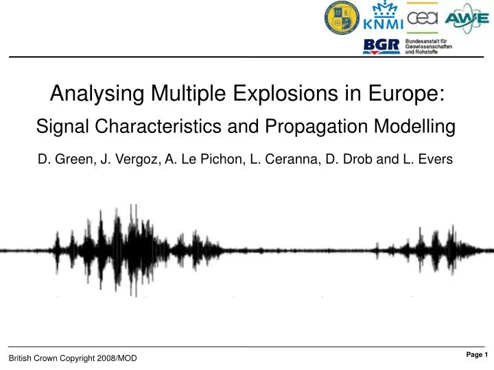
Analysing Multiple Explosions in Europe:. Signal Characteristics and Propagation Modelling. D. Green, J. Vergoz, A. Le Pichon, L. Ceranna, D. Drob and L. Evers. Analysing Multiple Explosions in Europe:. Signal Characteristics and Propagation Modelling.

E N D
Analysing Multiple Explosions in Europe: Signal Characteristics and Propagation Modelling D. Green, J. Vergoz, A. Le Pichon, L. Ceranna, D. Drob and L. Evers
Analysing Multiple Explosions in Europe: Signal Characteristics and Propagation Modelling D. Green, J. Vergoz, A. Le Pichon, L. Ceranna, D. Drob and L. Evers Summary • The 4 Explosion Series • Identifying Multiple Explosions • Gerdec Explosion • Observations • Propagation Modelling • Explosive Yield Estimation • Discussion / Conclusion
The Explosions Explosion IMS array (operational) Proposed IMS array Non-IMS array
Detections: F-Detector • Detections made using the F-detector (e.g., Blandford 1974) • Optimal detector for perfectly correlated signal in Gaussian, stationary noise • In presence of signal, F has a noncentral probability distribution • – can assign a probability that an F value is a detection at a given SNR. I26 Detections from Chelopechene Beam Filtered ( 0.3-0.8 Hz) F-Value Probability (SNR = 2)
Detections: F-Detector • Useful for picking signals out of a noisy background • Example below: signals at a range of 2097km recorded at BNIA (Blacknest) • Small aperture array (~200m), lots of cultural noise (roads) BNIA Detections from Chelopechene Beam Filtered (0.3-0.7 Hz) F-Value Probability (SNR = 5 )
Explosion Timings Expected Detections To the east To the west • Explosions occurred at times of strong stratospheric zonal wind • The detectibility along a given azimuth – controlled by along-path strato. wind
Gerdec Novaky Chelopechene Buncefield Observation Locations • Most observations as expected – downwind of source • Some exceptions – e.g., upwind arrival at I48TN from Gerdec • Downwind – signals have been detected at distances of over 4500km
Spectra Comparison: IS26 IS26: Detected all four explosions Note: • Gerdec – Power at >30s • Novaky – Upwind, very low SNR Yield Estimate (from period): (AFTAC eqn e.g., Edwards et al., 2006) (note comparison with pressure yields – p.24) Signal Noise
Multiple Explosion Observations Local Seismic Records • Find similar seismic signals • Assume: similar signal = • similar source at similar location • (λ/4 hypothesis) Gerdec TIR ~ 17km • Cross-correlate 1st six seconds • of P-wave. = master explosion = cross-correlation > 0.6 (all associated with above noise SNR) Chelopechene VTS ~ 25km Gerdec – 2 Explosions Chelopechene – 7 Explosions
Example of Observations: Chelopechene • Chelopechene – 03/07/2008 • All detections in westerly direction - as expected, Nth Hemisphere summer • Multiple arrivals from each explosion • Overlap of arrivals from first two • large explosions • A complex set of signals to explain. • - how to extract source information? • - what can we tell about propagation?
Multiple Explosion Observations • We want to: identify arrivals and compare different explosion signals. • Simplify by smoothing out fluctuations using envelope function (e.g., Dziewonski et al., 1969 ‘Multiple Filter Technique’) • Frequency-time plot can highlight small amplitude signals Narrowband Filtered (2.2-2.4 Hz) Signals at I48TN from Chelopechene, Bulgaria
Multiple Explosion Observations Signals at I48TN from Chelopechene, Bulgaria (Narrowband filter 2.2 – 2.4 to Hz applied) Overlapped Signals – use seismic arrivals as independent timebase Log10 Smoothed Envelope Waveforms
Multiple Explosion Observations Signals at I48TN from Chelopechene, Bulgaria I48TN I26DE (2.0-4.0 Hz) (0.4-3.0Hz) • Exp 2 36 minutes Exp 6 49 minutes Exp 7. Exp. 2 • At both stations early (fast) arrivals are missing from last • explosion (explosion 7). Exp. 6 Exp. 7
Gerdec Explosion - Observations • 6 infrasound observations • Observations through a wide • range of azimuths Backazimuths, uncorrected for wind deviations
Gerdec Explosion - Observations G2S I26DE (Germany) ECMWF • Perpendicular to dominant stratospheric wind dirn. • Ground-to-Stratosphere waveguides are weak, or • non-existent. I48TN (Tunisia) • Upwind arrivals observed from both explosions • Arrivals contain frequencies >1Hz and have arrival • times consistent with stratospheric arrivals.
Gerdec Explosion - Observations • Explosions separated by ~ 19 minutes • Very little difference between explosion • envelopes: • - arrival times almost identical • - small differences in relative amplitude
Propagation Modelling Available tools • Atmospheric Parameterisations - HWM, ECMWF, ARPEGE, G2S • Ray Tracing (1D to 3D) • Parabolic Equation Methods (Inframap) • Chebyshev Pseudospectral Method (L. Ceranna) Major Features to explain • Multiple infrasonic arrivals • Potentially upwind stratospheric arrivals • Temporal changes in waveforms
G2S – ECMWF – ARPEGE - HWM Atmospheric Parameterisations • - very similar up to altitudes of ~30km • significant differences in the stratosphere • what are the uncertainties in T,U and V? ECMWF and G2S Gerdec to IS26 (average profiles) G2S ECMWF HWM ARPEGE
Gerdec – Propagation Modelling Alt. (km) (@2Hz) dB re 1km -20 120 120 80 80 -60 40 40 0 -100 500 400 300 800 0 400 0 Eff. Sound Speed (m/s) Range (km) I26DE source Gerdec to IS26 (Germany) – PE model (J.Vergoz) • Very weak waveguide – difficult to explain the multiple (6) arrivals from each • explosion. Data
Gerdec – Propagation Modelling Gerdec to IS48 (Tunisia) – PE model (J. Vergoz) dB re 1km (@2Hz) Alt. (km) -60 120 120 80 80 -140 40 40 -220 0 0 400 300 1000 0 500 Eff. Sound Speed (m/s) Range (km) I48TN source • Elevated waveguide only • Little energy scattered/diffracted to ground Data
Gerdec – Propagation Modelling Alt. (km) 120 60 0 Gerdec to IS48 (Tunisia) – Chebyshev (L. Ceranna) Alt. (km) (@ 0.2Hz) 0 120 -20 60 dB -40 0 400 300 0 1000 2000 Eff. Sound Speed (m/s) Eff. Sound Speed (m/s) Range (km) I48TN source • Elevated waveguides – again diffracted arrivals return energy to the ground Data
Gerdec – Propagation Modelling Gerdec to IS48 (Tunisia) – Chebyshev (L. Ceranna) Cel. (km/s) Alt. (km) (@ 0.2Hz) 0 120 0.32 -20 0.28 60 0.24 dB -40 0 0 1000 2000 0 1000 2000 Range (km) Range (km) I48TN source • Elevated waveguides – again diffracted arrivals return energy to the ground • Correct celerity for observed arrivals Data
Propagation Issues Gerdec to IS26 (Germany) • How are the multiple arrivals generated? • - modelled waveguide is too weak • Would a narrow elevated waveguide generate the large number of arrivals? • How does energy leak down to the ground surface? Gerdec to IS48TN (Tunisia) • Propagation upwind – energy is trapped in an elevated waveguide • How does energy leak down to the ground surface?
Propagation Issues Gerdec to IS26 (Germany) Eff. Sound Speed (m/s) 2D and 3D structure • Preliminary investigations suggest that the 2D structure does not contain • significant changes in waveguide structure. Temporal Changes • Observed in data – unlikely to be resolved in models?
Yield Estimation • For the largest explosion of • each series. • Pressure corrected using • mean along-path wind values • at 50km altitude. • Ranges at particular stations • show the amplitude differences • between multiple arrivals for the • one explosion. Whitaker scaling relation used: (note comparison with pressure yields –p.9)
Yield Estimation – Multiple Exp. Chelopechene Gerdec • Only largest arrival shown on these plots • Consistent differences observed between stations: • - influence of : instrument calibration wind values taken from the model?
Conclusions / Further Studies • Four large explosion series (10-1000 tons TNT) have been well recorded • over the infrasound network in Europe and Asia. • Detections predominantly influenced by the stratospheric wind direction • - however propagation modelling does not always predict the correct number • of observed arrivals. • The Chelopechene explosion series suggests that explosions of down to a few • tonnes of high explosive equivalent can be recorded at stations ~1000km distant • from the source. • Downwind of the large explosions, detections can be made at over 4500km from • the source. Future Improvements • Propagation path identification • If the atmospheric models cannot explain the arrivals, what information • can we use to identify the most probable path? • Temporal signal changes - What do these tell us about the atmospheric variability?
Atmospheric Slices – Gerdec to I26 Eff. Sound Speed (m/s) • ECMWF and G2S – almost identical up to 25km altitude • Significant differences (~ 10 m/s) within the stratosphere • What are the uncertainities?
Aside: Tropospheric Interaction Large tropospheric signals for Buncefield - due to influence of temperature inversion?
Observation Locations Not Observed Observed Buncefield Novaky Chelopechene Gerdec Wind vectors from HWM = 100m/s
Discussion / Possible Scenarios • Can the strength of a given elevated waveguide influence the temporal • evolution of the observed signals? • If an elevated waveguide weakens – the first signals to be removed are the • low angle of incidence rays – these correspond to the fast arrivals.