Download
1 / 26

E N D
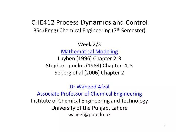
CHE412 Process Dynamics and ControlBSc (Engg) Chemical Engineering (7th Semester)Week 2/3Mathematical ModelingLuyben (1996) Chapter 2-3 Stephanopoulos (1984) Chapter 4, 5Seborg et al (2006) Chapter 2DrWaheedAfzal Associate Professor of Chemical Engineering Institute of Chemical Engineering and TechnologyUniversity of the Punjab, Lahorewa.icet@pu.edu.pk
Test yourself (and Define): • Stability • Block diagram • Transducer • Final control element • Mathematical model • Input-out model, transfer function • Deterministic and stochastic models • Optimization • Types of Feedback Controllers (P, PI, PID) • Dynamics (of openloop and closedloop) systems • Manipulated Variables • Controlled/ Uncontrolled Variables • Load/Disturbances • Feedback, Feedforward and Inferential controls • Error • Offset (steady-state value of error) • Set-point Hint: Consult recommended books (and google!) Luyben (1996), Coughanower and LeBlanc (2008)
Types of Feedback Controllers • Proportional: c(t) = KcЄ(t) + cs • Proportional-Integral: • Proportional-Integral-Derivative: Nomenclature actuating output , error , gain , time constant Consult your class notes on modelling of stirred tank heater (t) (Stephanopoulos, 1984)
Mathematical Modeling • Mathematical representation of a process (chemical or physical) intended to promote qualitative and quantitative understanding • Set of equations • Steady state, unsteady state (transient) behavior • Model should be in good agreement with experiments Experimental Setup Inputs Outputs Compare Set of Equations (process model) Outputs
Systematic Approach for Modelling (Seborg et al 2004) • Determine objectives, end-use, required details and accuracy • Draw schematic diagram and label all variables, parameters • Develop basis and list all assumptions; simplicity Vs reality • If spatial variables are important (partial or ordinary DEs) • Write conservation equations, introduce auxiliary equations • Never forget dimensional analysis while developing equations • Perform degree of freedom analysis to ensure solution • Simplify model by re-arranging equations • Classify variables (disturbances, controlled and manipulated variables, etc.)
Need of a Mathematical Model • To understand the transient behavior, how inputs influence outputs, effects of recycles, bottlenecks • To train the operating personnel (what will happen if…, ‘emergency situations’, no/smaller than required reflux in distillation column, pump is not providing feed, etc.) • Selection of control pairs (controlled v. / manipulated v.) and control configurations (process-based models) • To troubleshoot • Optimizing process conditions (most profitable scenarios)
Classification of Process Models based on how they are developed • Theoretical Models based on principal of conservation- mass, energy, momentum and auxiliary relationships, ρ, enthalpy, cp, phase equilibria, Arrhenius equation, etc) • Empirical model based on large quantity of experimental data) • Semi-empirical model (combination of theoretical and empirical models) Any available combination of theoretical principles and empirical correlations
Advantages of Different Models • Theoretical Models • Physical insight into the process • Applicable over a wide range of conditions • Time consuming (actual models consist of large number of equations) • Availability of model parameters e.g. reaction rate coefficient, over-all heart transfer coefficient, etc. • Empirical model • Easier to develop but needs experimental data • Applicable to narrow range of conditions
State Variables and State Equations • State variables describe natural state of a process • Fundamental quantities (mass, energy, momentum) are readily measurable in a process are described by measurable variables (T, P, x, F, V) • State equations are derived from conservation principle(relates state variables with other variables) (Rate of accumulation) = (rate of input) – (rate of output) + (rate of generation) - (rate of consumption)
Modeling ExamplesJacketed CSTR Fi, CAi, Ti • Basis Flow rates are volumetric Compositions are molar A → B, exothermic, first order • Assumptions Perfect mixing ρ, cP are constant Perfect insulation Coolant is perfectly mixed No thermal resistance of jacket F, CA, T Coolant
Modeling of a Jacketed CSTR (Contd.) Fi, CAi, Ti • Overall Mass Balance (Rate of accumulation) = (rate of input) – (rate of output) • Component Mass Balance (Rate of accumulation of A) = (rate of input of A) – (rate of output of A) + (rate of generation of A) – (rate of consumption of A) Coolant Fco,Tco V CA T F, CA, T • Energy Balance • (Rate of energy accumulation) = (rate of energy input) – (rate of energy output) - (rate of energy removal by coolant) + (rate of energy added by the exothermic reaction) Coolant Fci,Tci
Modeling of a Jacketed CSTR (Contd.) Fi, CAi, Ti • Overall Mass Balance • Component Mass Balance • Energy Balance Coolant Fco,Tco V CA T F, CA, T Input variables: CAi, Fi, Ti, Q, (F) Output variables: V, CA, T Coolant Fci,Tci
Degrees of Freedom (Nf) Analysis Nf = Nv - NE Case (1): Nf = 0 i.e. Nv = NE (exactly specified system) We can solve the model without difficulty Case (2): f > 0 i.e. Nv > NE(under specified system), infinite number of solutions because Nf process variables can be fixed arbitrarily. either specify variables (by measuring disturbances) or add controller equation/s Case (3): Nf < 0 i.e. Nv < NE (over specified system) set of equations has no solution remove Nf equation/s We must achieve Nf = 0 in order to simulate (solve) the model
Stirred Tank Heater: Modeling and Degree of Freedom Analysis Basis/ Assumptions • Perfectly mixed, Perfectly insulated • ρ, cPare constant • Overall Mass Balance • Energy Balance A Steam Fst • Degree of Freedom Analysis • Independent Equations: 2 Variables: 6 (h, Fi, F, Ti, T, Q) • Nf= 6-2 (= 4) Underspecified
Stirred Tank Heater: Modeling and Degree of Freedom Analysis Nf = 4 • Specify load variables (or disturbance) Measure Fi, Ti (Nf = 4 - 2 = 2) • Include controller equations (not studied yet); specify CV-MV pairs: A Steam Fst Nf = 2 - 2 = 0 Can you draw these control loops?
Modeling an Ideal Binary Distillation Column Condenser Basis/ Assumptions • Saturated feed • Perfect insulation of column • Trays are ideal • Vapor hold-up is negligible • Molar heats of vaporization of A and B are similar • Perfect mixing on each tray • Relative volatility (α) is constant • Liquid holdup follows Francis weir formulae • Condenser and Reboiler dynamics are neglected • Total 20 trays, feed at 10 2, 4, 5 → V1 = V2 = V3 = … VN (not valid for high-pressure columns) = 20 Reflux Drum mD F Z D xD R xD VB mB Reboiler B xB (Stephanopoulos, 1984)
Modeling Distillation Column V20 Reflux Drum • Overall • Component mD D xD R xD Top Tray • Overall • Component ) Remember V1 = V2 = …. VN = VB Reflux Drum V20 R N = 20 V19 L20 Top Tray
Modeling Distillation Column LN+1 L11 vN v10 F Z mN mN Nth Stage (stages 19 to 11 and 9 to 2) • Overall • Component …. simplify! Feed Stage (10th) Nth Stage LN L10 vN-1 v9 Feed Stage (10th) • Overall • Component …. simplify!
Modeling Distillation Column 1st Stage • Overall • Component … simplify! 1st Stage V1 L2 L1 L1 VB VB Column Base • Overall • Component …. simplify! mB VB Column Base B
Modeling Distillation Column Equilibrium relationships (to determine y) • Mass balance (total and component) around 6 segments of a distillation column: reflux drum, top tray, Nth tray, feed tray, 1st tray and column base. • Solution of ODE for total mass balance gives liquid holdups (mN) • Solution of ODE for component mass balance gives liquid compositions (xN) • V1 = V2 = … = VN = VB (vapor holdups) • How to calculate y (vapor composition) and L (liquid flow rate) • Recall αij is constant throughout the column • Use αij= ki/kj , xi + xj =1,yi + yj = 1, and k = y/x to prove Phase-equilibrium relationship (recall thermodynamics)
Modeling Distillation Column Hydraulic relationships (to determine L) • Liquid flow rate can be calculated using well-known Francis weir hydraulic relationship; simple form of this equation is linearized version: • LN is flow rate of liquid coming from Nth stage • LN0is reference value of flow rate LN • mNis liquid holdup at Nth stage • mN0is reference value of liquid holdup mN • β is hydraulic time constant (typically 3 to 6 seconds)
Modeling Distillation Column Degree of Freedom Analysis Total number of independent equations: • Equilibrium relationships (y1, y2, …yN, yB) →N+1 (21) • Hydraulic relationships (L1, L2, …LN) → N (20) (does not work for liquid flow rates D and B) • Total mass balances (1 for each tray, reflux drum and column base)→ N+2(22) • Total component mass balances (1 for each tray, reflux drum and column base) → N+2(22) • Total Number of equations NE = 4N + 5 (85) 44 differential and 41 algebraic equations Note the size of model even for a ‘simple’ system with several simplifying assumptions!
Modeling Distillation Column Degree of Freedom Analysis Total number of independent variables: • Liquid composition (x1, x2, …xN, xD,xB) →N+2 • Liquid holdup (m1, m2, …mN, mD,mB) →N+2 • Vapor composition (y1, y2, …yN, yB) →N+1 • Liquid flow rates (L1, L2, …LN) →N • Additional variables → 6 (Feed: F, Z; Reflux: D, R; Bottom: B, VB) • Total Number of independent variables NV = 4N + 11 Degree of Freedom = (4N + 11) – (4N + 5) = 6 System is underspecified
Modeling Distillation Column Degree of Freedom Analysis (4N + 11) – (4N + 5) = 6 • Specify disturbances: F, Z (Nf = 6-2 = 4) • Include controller equations (Recall our discussion on types of feedback controllers ) • General form, of P-Controller c(t) = cs+ KcЄ(t) Controller Equation (Proportional Controller) R = Kc (xs- xD) + Rs VB = Kc (xBs-xB) + VBs D = Kc (mDs-mD) + Ds B = Kc (mBs-mB) + Bs Nf= 4 - 4 = 0 Can you draw these four feedback control loops?
Feedback Control on a Binary Distillation Column R (Stephanopoulos, 1984)
Week 2/3Weekly Take-Home Assignment • Define all the terms on slide 2 with examples whenever possible. • Prepare short answers to ‘things to think about’ (Stephanopoulos, 1984) page 33-35 • Prepare short answers to ‘things to think about’ (Stephanopoulos, 1984) page 78-79 • Solve the following problems (Chapter 4 and 5 of Stephanopoulos, 1984): II.1 to II.14, II.22, II.23 (Compulsory) Submit before Friday Curriculum and handouts are posted at: http://faculty.waheed-afzal1.pu.edu.pk/