Download

1 / 44
450 likes | 688 Views
The Network Layer. Chapter 5. Network Layer Design Isues. Store-and-Forward Packet Switching Services Provided to the Transport Layer Implementation of Connectionless Service Implementation of Connection-Oriented Service Comparison of Virtual-Circuit and Datagram Subnets.

E N D
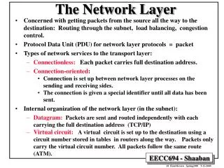
The Network Layer Chapter 5
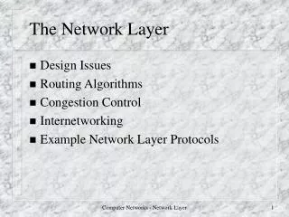
Network Layer Design Isues • Store-and-Forward Packet Switching • Services Provided to the Transport Layer • Implementation of Connectionless Service • Implementation of Connection-Oriented Service • Comparison of Virtual-Circuit and Datagram Subnets
Store-and-Forward Packet Switching fig 5-1 The environment of the network layer protocols.
Implementation of Connectionless Service Routing within a diagram subnet.
Implementation of Connection-Oriented Service Routing within a virtual-circuit subnet.
Routing Algorithms • The Optimality Principle • Shortest Path Routing • Flooding • Distance Vector Routing • Link State Routing
Optimality principleBellman concept 1 2 i If node i is on the minimal path (1,2) then: path(1,i) is minimal and path(i,2) is minimal.
A sink tree for router B A sink tree for router B A subnet
Dijkstra: shortest path A to D • Mark A permanent and calculate distance to the neighbors (B and G). • Mark the smallest node (B) permanent and calculate neighbor distance • from it. If you hit a conflict choose smaller distance. • Do step 2 until all network is covered.
Dijkstra's algorithm 5-8 top
Dijkstra's algorithm (2) 5-8 bottom
Dijkstra 5 D(5,A) B(2,A) 3 5 2 3 A F 2 1 5 1 2 D(4,C) B(2,A) 3 1 E 5 2 C(1,A) 5 3 A F 2 1 D(3,E) B(2,A) 1 2 3 5 1 2 3 C(1,A) A E(2,C) 2 1 1 F(4,E) 2 1 5 D(3,E) B(2,A) E(2,C) C(1,A) 3 5 2 F(8,D) 3 A 2 1 1 F(4,E) 2 1 E(2,C) C(1,A) 5 D(3,E) B(2,A) 3 5 2 F(8,D) 3 A 2 1 1 F(4,E) 2 1 E(2,C) C(1,A)
Bellman-Ford = Distant vector = RIP(example) 5 (-1,oo) (-1,oo) 3 2 3 5 2 3 1 6 initial 2 1 1 (-1,oo) 2 (-1,0) 1 4 5 (-1,oo) (-1,oo) 5 (1,5,1) (1,2,1) 3 2 3 Number of hops h=1 5 2 3 1 6 2 1 1 2 (-1,0,0) (-1, oo, oo) 1 4 5 (-1, oo, oo) (1,1,1) (predecessor , dmin , no of hops)
Bellman-Ford example (2) 5 3 5 2 3 2 2 3 4 5 6 1 2 1 (2,5,2) (4,4,2) (1,5,1) (1,2,1) (3,8,2) (4,3,2) h=2 1 1 (3,10,2) (-1,0,0) (1,1,1) (4,2,2) (3,8,2) (3,6,2) (2,4,2) 5 (1,2,1) (4,4,2) 3 h<=2 2 3 5 2 3 1 6 2 1 1 (3,10,2) 2 (-1,0,0) 1 4 5 (1,1,1) (4,2,2)
Bellman-Ford example (3) 5 3 5 2 3 2 6 4 3 2 5 1 2 1 (1,2,1) (3,7,3) (4,4,2) (5,3,3) h=3 1 1 (3,10,2) (-1,0,0) (3,9,3) (5,4,3) (1,1,1) (4,2,2) (6,12,3) (3,5,3) (5,3,3) 5 (1,2,1) (5,3,3) 3 h<=3 2 3 5 2 3 1 6 2 1 1 2 (-1,0,0) (5,4,3) 1 4 5 (1,1,1) (4,2,2)
Bellman-Ford example (4) 5 3 5 2 3 2 3 4 2 6 5 1 2 1 (6,9,4) (5,3,3) (1,2,1) h=4 1 1 (5,4,3) (-1,0,0) (3,8,4) (1,1,1) (4,2,2) (6,6,4) (3,4,4) (1,2,1) (5,3,3) 3 h<=4 2 3 5 2 3 1 6 2 1 1 (5,4,3) 2 (-1,0,0) 1 4 5 (1,1,1) (4,2,2)
Bellman-Ford example (5) 5 (1,2) (5,3) 3 final 2 3 5 2 3 1 6 2 1 1 2 (5,4) (-1,0) 1 4 5 (1,1) (4,2)
Distance Vector Routing one hop matrix h=1 two hops matrix h=2 * = • Algorithm: • N1(i,k) * N1(k,j) = mink (m(i,k)+n(k,j)) = N2(i,j) • N<2(i,j) = min(N1(i,j), N2(i,j)) • Proceed steps 1. and 2. up to the M = dept of the network.
Distance Vector Routing in practice (a) A subnet. (b) Input from A, I, H, K, and the new routing table for J.
Distance Vector Routing (2) The count-to-infinity problem.
Link State Routing Each router must do the following: • Discover its neighbors, learn their network address. • Measure the delay or cost to each of its neighbors. • Construct a packet telling all it has just learned. • Send this packet to all other routers. • Compute the shortest path to every other router.
Learning about the Neighbors (a) Nine routers and a LAN. (b) A graph model of (a).
Measuring Line Cost A subnet in which the East and West parts are connected by two lines.
Building Link State Packets (a) A subnet. (b) The link state packets for this subnet.
Distributing the Link State Packets The packet buffer for router B in the previous slide (Fig. 5-13).
Hierarchical Routing Hierarchical routing.
Broadcast Routing Reverse path forwarding. (a) A subnet. (b) a Sink tree. (c) The tree built by reverse path forwarding.
Multicast Routing (a) A network. (b) A spanning tree for the leftmost router. (c) A multicast tree for group 1. (d) A multicast tree for group 2.
Routing for Mobile Hosts A WAN to which LANs, MANs, and wireless cells are attached.
Routing for Mobile Hosts (2) Packet routing for mobile users.
Routing in Ad Hoc Networks Possibilities when the routers are mobile: • Military vehicles on battlefield. • No infrastructure. • A fleet of ships at sea. • All moving all the time • Emergency works at earthquake . • The infrastructure destroyed. • A gathering of people with notebook computers. • In an area lacking 802.11.
Route Discovery • (a) Range of A's broadcast. • (b) After B and D have received A's broadcast. • (c) After C, F, and G have received A's broadcast. • (d) After E, H, and I have received A's broadcast. Shaded nodes are new recipients. Arrows show possible reverse routes.
Route Discovery (2) Format of a ROUTE REQUEST packet.
Route Discovery (3) Format of a ROUTE REPLY packet.
Route Maintenance (a) D's routing table before G goes down. (b) The graph after G has gone down.
Node Lookup in Peer-to-Peer Networks (a) A set of 32 node identifiers arranged in a circle. The shaded ones correspond to actual machines. The arcs show the fingers from nodes 1, 4, and 12. The labels on the arcs are the table indices. (b) Examples of the finger tables.
Congestion Control Algorithms • General Principles of Congestion Control • Congestion Prevention Policies • Congestion Control in Virtual-Circuit Subnets • Congestion Control in Datagram Subnets • Load Shedding • Jitter Control
Congestion When too much traffic is offered, congestion sets in and performance degrades sharply.
General Principles of Congestion Control • Monitor the system . • detect when and where congestion occurs. • Pass information to where action can be taken. • Adjust system operation to correct the problem.
Congestion Prevention Policies 5-26 Policies that affect congestion.
Congestion Control in Virtual-Circuit Subnets (a) A congested subnet. (b) A redrawn subnet, eliminates congestion and a virtual circuit from A to B.
Hop-by-Hop Choke Packets (a) A choke packet that affects only the source. (b) A choke packet that affects each hop it passes through.
Jitter Control (a) High jitter. (b) Low jitter.