Download
1 / 100
1k likes | 1.02k Views
The Network Layer. Concerned with getting packets from the source all the way to the destination: Routing through the subnet, load balancing, congestion control. Protocol Data Unit (PDU) for network layer protocols = packet Types of network services to the transport layer:

E N D
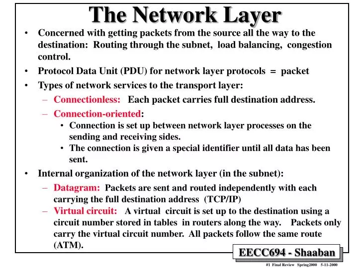
The Network Layer • Concerned with getting packets from the source all the way to the destination: Routing through the subnet, load balancing, congestion control. • Protocol Data Unit (PDU) for network layer protocols = packet • Types of network services to the transport layer: • Connectionless: Each packet carries full destination address. • Connection-oriented: • Connection is set up between network layer processes on the sending and receiving sides. • The connection is given a special identifier until all data has been sent. • Internal organization of the network layer (in the subnet): • Datagram:Packets are sent and routed independently with each carrying the full destination address (TCP/IP) • Virtual circuit:A virtual circuit is set up to the destination using a circuit number stored in tables in routers along the way. Packets only carry the virtual circuit number. All packets follow the same route (ATM).
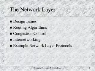
Routing Algorithms To decide which output line an incoming packet should be transmitted on. • Static Routing (Nonadaptive algorithms): • Shortest path routing: • Build a graph of the subnet with each node representing a router and each arc representing a communication link. • The weight on the arcs represents: a function of distance, bandwidth, communication costs mean queue length and other performance factors. • Several algorithms exist including Dijkstra’s shortest path algorithm. • Selective flooding: Send the packet on all output lines going in the right direction to the destination. • Flow-based routing: Based on known capacity and link loads.
Static Routing: Shortest Path Routing • First five steps of an example using Dijktra’s algorithm
Static Routing: Flow-Based Routing • A routing matrix is constructed; used when the mean data flow in network links is known and stable. • Given: Capacity matrix Cij, Traffic matrix Fij, • Mean delay at each line T= 1/(mC -l) mC line capacity packet/sec l traffic packet/sec A subnet with link capacities given in kbps The traffic in packets/sec and routing table
Flow-Based Routing Calculation Example Flow-based routing analysis example for network on previous page, assuming: Mean packet size = 800 bits Reverse traffic is the same as forward traffic weighti = flow in link i / total flow in the subnet Mean delay per packet = åweighti x Ti = 86 msec in above example Goal find a flow with minimum mean delay per packet.
Used in ARPANET until 1979 Dynamic Routing: Distance Vector • Each router maintains a table with one entry for each router in the subnet including the preferred outgoing link, and an estimate of time or distance to the destination router. • Neighbor router table entries are gathered by sending ECHO packets which are sent back with a time stamp. • Each router exchanges its table of estimates with its neighbors; the best estimate is chosen.
Distance Vector Routing: Count-to-Infinity Problem Link AB Initially down The main reason Distance Vector Routing has been mostly abandoned Link AB Initially Up
Dynamic Routing: Link State Routing • Resolves Count-to-Infinity Problem present in Distance Vector Routing. • Variants of link state routing are widely used. • Each router using Link State Routing must: • Discover its neighbors and know their network address • Measure the delay or cost to each of the neighbors using ECHO packets. • Construct a link state packet to include what it learned about its neighbors including the age of the information. • Send the link state packet to all other routers in the subnet • Compute the shortest path to every other router based on information gathered from all link state packets (Dijksra’a algorithm may be used).
Hierarchical Routing • The subnet is divided into several regions of routers. • Each router maintains a table of routing information to routers in its region only. • Packets destined to another region are routed to a designated router in that region. A two-level Hierarchical Routing Example: Optimum number of hierarchy levels: For a subnet of N routers: Optimum # of levels = ln N Total # of table entries = e ln N
Congestion Control Methods • Traffic Shaping: • Heavily used in VC subnets including ATM networks. • Avoid bursty traffic by producing more uniform output at the hosts. • Representative examples: Leaky Bucket, Token Bucket. • Admission Control: • Used in VC subnets. • Once congestion has been detected in part of the subnet, no additional VCs are created until the congestion level is reduced. • Choke Packets: • Used in both datagram and VC subnets • When a high level of line traffic is detected, a choke packet is sent to source host to reduce traffic. • Variation Hop-by-Hop choke packets. • Load Shedding: • Used only when other congestion control methods in place fail. • When capacity is reached, routers or switches may discard a number of incoming packets to reduce their load.
Congestion Control Algorithms: The Leaky Bucket • A traffic shaping method that aims at creating a uniform transmission rate at the hosts. • Used in ATM networks. • An output queue of finite length is connected between the sending host and the network. • Either built into the network hardware interface or implemented by the operating system. • One packet (for fixed-size packets) or a number of bytes (for variable-size packets) are allowed into the queue per clock cycle. • Congestion control is accomplished by discarding packets arriving from the host when the queue is full.
Congestion Control Algorithms: The Token Bucket • An output queue is connected to the host where tokens are generated and a finite number is stored at the rate of DT • Packets from the host can be transmitted only if enough tokens exist. • When the queue is full tokens are discarded not packets. • Implemented using a variable that counts tokens.
Congestion Control Algorithms: Choke Packets • Used in both VC and datagram subnets. • A variable “u” is associated by the router to reflect the recent utilization of an output line: u = auold + (1 - a) f • When “u” goes above a given threshold, the corresponding line enters a warning state. • Each new packet is checked if its output line is in warning state if so: • The router sends a choke packet to the source host with the packet destination. • The original packet is tagged (no new choke packets are generated). • A host receiving a choke packet should reduce the traffic to the specified destination • A variation (Hop-by-Hop Choke Packets) operate similarly but take effect at each hop while choke packets travel back to the source.
INTERNETWORKING • When several network types with different media, topology and protocols, are connected to form a larger network: • UNIX: TCP/IP • Mainframe networks: IBM’s SNA, DEC’s DECnet • PC LANs: Novell: NCP/IPX, AppleTalk • ATM, wireless networks etc. • The “black box” converter unit used to connect two different networks depend on the layer of connection: • Layer 1 (physical): Repeaters, bit level • Layer 2 (data link): Bridges, data link frames • Layer 3 (network): Multiprotocol routers, packets • Layer 4 (transport): Transport gateways • Above 4 (application): Application gateways.
Internetworking Issues:Fragmentation • When packets from a subnet travel to another subnet with a smaller maximum packet size, packets have to be broken down into fragments and send them as internet packets. Transparent fragmentation Host Non-transparent fragmentation
The Internet • Evolved from the ARPANET (the Advanced Research Projects Agency Network), a project funded by The U.S. Department of Defense (DOD) in 1969. • ARPANET's purpose was to provide the U.S. Defense Network (DDN) with redundant links between its sites and the Pentagon, relying on intelligent data packets that could automatically route themselves around failed network routers and links. • During the 1970s, the ARPANET gradually transformed and expanded into the current Internet as new protocols and technologies became available, and as additional defense, research, scientific, commercial and development organizations were added to the network. • At the network layer level: The Internet is a global collection of subnets held together by a common main network layer protocol: IP (Internet Protocol). • Example Transport Layer Protocols: • Connection-oriented: TCP (Transport Control Protocol), • Connectionless: UDP (User Data Protocol)
Classic IP Addressing Architecture • The classical IP network prefix is the Class A, B, C, D, or E network prefix. • These address ranges are discriminated by observing the values of the most significant bits of the address, and break the address into simple network prefix (or number) and host number fields: IP-address ::= { <Network-prefix>, <Host-number> } • The network classes are identified as follows: • 0xxx Class A general purpose unicast addresses with standard 8 bit prefix. • 10xx Class B general purpose unicast addresses with standard 16 bit prefix. • 110x Class C general purpose unicast addresses with standard 24 bit prefix. • 1110 Class D IP Multicast Addresses - 28 bit prefix, non-aggregatable • 1111 Class E reserved for experimental use. • To allow hierarchical routing, an IP address can be further divided : • IP-address ::= { <Network-number>, <Subnet-number>, <Host-number> } • The interconnected physical networks within an organization use the same network prefix but different subnet numbers. • Routers outside the network treat <Network-prefix> and <Host-number> together as an uninterpreted part of the 32-bit IP address.
Max # of class A networks = 27 - 2 = 126 networks each containing 224 -2 = 16,777,214 host addresses 50% of the total IPv4 unicast address space Max # of class B networks = 214 = 16,384 networks each containing 216 -2 = 65,534 host addresses 25% of the total IPv4 unicast address space Max # of class C networks = 221 = 2,097,152networks each containing 28 -2 = 254 host addresses 12.5% of the total IPv4 unicast address space Primary IP Primary Address Classes Growth of Internet Routing Tables Allocated Network Numbers By Class
Network Mask • A 32-bit number indicating the range of IP addresses residing on a single IP network/subnet/supernet and the length of the network-prefix. • For example, the network mask for a class C IP network is given as 255.255.255.0 • To identify the network/subnet of a destination IP address, routers logically AND the mask and the full destination IP address then compare the result with network addresses in routing table to determine the next hop. • One of the fundamental features of IP addressing is that each address contains a self-encoding key that identifies the dividing point between the network-prefix and the host-number. • For example, if the first two bits of an IP address are 1-0, the dividing point falls between the 15th and 16th bits. • This simplified the routing system during the early years of the Internet because the original routing protocols did not supply a "mask" with each route to identify the length of the network-prefix.
Internet Control Message Protocol (ICMP) • ICMP is an Internet network protocol that provides an error-reporting mechanism. • Usually used by routers to report unexpected events and errors and to measure delays (ping), explore new routers and routes (traceroute). • ICMP messages are encapsulated in IP packets: • When reporting an error, router sends message back to source in an ICMP datagram message contains information about problem. • Ping program uses ICMP echo request and echo reply messages sent by host to test if the target host is reachable.
Routing In The Internet • TCP/IP Networks and LANs: • The Address Resolution Protocol (ARP). • Table Lookup Address Resolution. • Reverse Address Resolution Protocol (RARP) • Internal Routing in Autonomous systems: • Link state based Open Shortest Path First (OSPF). Routing. • External routing between Autonomous systems: • Exterior gateway protocol: Border Gateway Protocol (BGP). • Classless Inter-Domain Routing (CIDR).
The Address Resolution Protocol (ARP) • Address resolution: Finding hardware address that corresponds to a network layer protocol address. • In Ethernet-based LANs, each machine connected to the LAN has a unique flat 48 bit Ethernet address encoded in its NIC by the manufacturer. • ARP: When the transport layer on a LAN-connected machine passes a message to be transmitted to the IP layer and destined to another machine on the LAN: • Translate the host name of the receiver to its IP address using the Domain Name System (DNS). • Broadcast a packet to the LAN requesting the Ethernet address of the machine with the given IP (step 1 of ARP). • The target machine with this IP replies with its Ethernet address E (step 2 of ARP). • IP software on the source machine builds an Ethernet frame with Ethernet address E and puts the IP packet its payload field. • The destination machine picks up the Ethernet frame and extracts and passes the IP packet to its IP software.
A portion of an IP/Ethernet address resolution table Table Lookup Address Resolution • A table containing the IP address and hardware address of each host on the LAN and its corresponding hardware (Ethernet) address is used. • When sending frames to another host on the LAN, the table is searched on the IP address and the corresponding hardware address in the table is found. • Often used in conjunction with ARP to reduce address resolution overhead: • The table initially cleared at system startup . • For every host with no entry in the table ARP is used to find its hardware address. • The corresponding hardware address obtained from ARP is added or cached in the sending host’s table. • Table entries are periodically discarded to prevent stale addresses.
Reverse Address Resolution Protocol (RARP) • Used by machines joining the network, with no IP address stored in the machine, to find out the assigned IP addresses corresponding to the machine’s Ethernet NIC addresses. • Such a machine broadcasts a request with its Ethernet address using RARP. • The RARP server on the LAN replies to the request with the IP address from its configuration files. • RARP broadcasts are limited to a LAN and not forwarded to routers ®Each LAN must have an RARP server. • Bootstrap protocol BOOTP: Uses UDP packets which can be forwarded to routers ® No need for a BOOTP server on each LAN.
Routing In The Internet • The Internet as a whole is formed from a number of AutonomousSystems. • Each AS is further divided into areas with a special area 0 (the backbone) connected to all its other areas. • Internal routing in an AS is handled by an interior gateway protocol: Open Shortest Path First (OSPF), a hierarchical, dynamic link-state routing algorithm which supports: • Point-to-point connection between two routers. • Multi-access networks, with broadcasting (LANS ), and without (WANS). • External routing between ASes is handled by an exterior gateway protocol: Border Gateway Protocol (BGP): • The network is reduced to BGP routers and their links. • Based on a distance vector protocol with actual path used being exchanged between routers.
Open Shortest Path First (OSPF) • OSPF is a TCP/IP link-state based Internet routing protocol designed to run internal to a single Autonomous System. • IP packets are routed based solely on the destination IP address found in the IP packet header without adding further protocol headers. • Each OSPF router maintains an identical link-state database describing the router's usable interfaces, reachable neighbors and the Autonomous System's topology. • From this database, a routing table is initially calculated by constructing a shortest-path tree. • When several equal-cost routes to a destination exist, traffic is distributed equally among them. • Topological changes in the AS (such as router interface failures) are quickly detected by calculating new loop-free routes. • Each router distributes its local state throughout the Autonomous System by flooding. • Sets of networks may be grouped together in an area where the topology of an area is hidden from the rest of the Autonomous System.
AS 1 AS 2 Backbone Backbone router Area Internal router EGP protocol connects the ASes AS 4 AS 3 Area border router AS boundary router The Relation Between: ASes, Backbones and Areas in OSPF
Border Gateway Protocol (BGP) • BGP is intended for use between networks owned by different organizations (Backbone Providers). • BGP is often referred to as a tool for "policy" routing, because • It may not take into account network constraints such as available bandwidth or network load. • The primary routing protocol that Internet backbone providers use to exchange routing information. • Each provider will configure its border routers to announce certain routes to its neighbors. • The neighboring provider will filter those announcements based on its own policies and will discard some of those announced routes. • Of the routes that are accepted, some may only be used locally, in the provider's own routing tables, and some may be announced to other neighboring backbones.
Classless Inter-Domain Routing (CIDR) • Eliminates the traditional concept of Class A, Class B, and Class C network addresses, replacing them a generalized concept of a "network-prefix." • Supports route aggregation where a single routing table entry can represent the address space of perhaps thousands of traditional class network routes. • Without the rapid deployment of CIDR in 1994 and 1995, the Internet routing tables would have been in excess of 70,000 routes (instead of the current 30,000+). • A prefix-length is included with each piece of routing information. The prefix-length is a way of specifying the number of leftmost contiguous bits in the network-portion of each routing table entry. • For example, a network with 20 bits of network-number and 12-bits of host-number would have with a 20-bit prefix length, which could be a former Class A, Class B, or Class C. • Routers that support CIDR do not make assumptions based on the first 3-bits of the address, they rely on the prefix-length information provided with the route.
Asynchronous Transfer Mode (ATM) • ATM is a specific asynchronous packet-oriented information, multiplexing and switching transfer model standard, originally devised for digital voice and video transmission, which is • Based on 53-byte fixed-length cells. • Each cell consists of a 48 byte information field and a 5 byte header, which is mainly used to determine the virtual channel and to perform the appropriate routing. • Cell sequence integrity is preserved per virtual channel. Thus all cells belonging to a virtual channel must be delivered in their original order. • Original primary rate: 155.52 Mbps. Additional rate: 622.08 Mbps • ATM is connection-oriented. • Header values including virtual path/circuit numbers are assigned to each section of a connection for the complete duration of the connection. • The information field of ATM cells is carried transparently through the network. No processing like error control is performed on it inside the network. • All services (voice, video, data, ) can be transported via ATM, including connectionless services. • To accommodate various services an appropriate adaptation layer is provided to fit information of all services into ATM cells and to provide service specific functions (e.g. clock recovery, cell loss recovery, ...).
Virtual Circuits • When a virtual circuit is established: • The route is chosen from beginning to end (circuit setup needed). • Routers or switches along the circuit create table entries used to route data transmitted on the virtual circuit. • Permanent virtual circuits - Switched virtual circuits
Fixed cell size = 53 bytes Input side Output side ATM Cells & Switches ATM Cell Format Cell Duration: ~ 2.7 msecfor 155.52 Mbps ATMs ~ 700 nsec for 622.08 Mbps ATMs An ATM switch
ATM Layer Headers ATM layer header at User-Network Interface UNI ATM layer header at Network-Network Interface NNI
The Network Layer In ATM Networks • The ATM layer handles the functions of the network layer: • Moving cells from source to destination in order. • Routing algorithms within ATM switches, global addressing. • Connection-oriented without acknowledgments. • The basic element is the unidirectional virtual circuit or channel with fixed-size cells. • Two possible interfaces: • UNI (User-Network Interface): Boundary between an ATM network and host. • NNI (Network-Network Interface): Between two ATM switches (or routers).
ATM Network Connection Setup/Release Connection Setup Connection Release
ATM Virtual Path Re-routing Example Rerouting a virtual path re-routes all of its virtual circuits
ATM Routing Example Possible routes through the Omaha ATM switch
ATM Routing Example: Table Entries Table entries corresponding to routes through the Omaha ATM switch
ATM Switch Functions • The main function of an ATM switch is to relay user data cells from input ports to the appropriate output ports. The switch processes only user data cell headers and the payload is carried transparently. • As soon as the cell comes in through the input port, Virtual Path/Channel Identifiers (VPI/VCI) information is extracted from the cell and used to route the cells to the appropriate output port. • This function can be divided into three functional blocks: the input module at the input port, the cell switch fabric (or switch matrix) that performs the actual routing, and the output modules at the output ports. • Establishment and control of the VP/VC connections. • Unlike user data cells, information in signaling or control cells payload is not transparent to the network. • The switch identifies signaling cells, and even generates some itself. • Connection Admission Control (CAC) carries out the major signaling functions required. • Signaling/control information may not pass through the cell switch fabric, and instead is exchanged through a separate signaling network. • Network management functions, concerned with monitoring the controlling the network to ensure its correct and efficient operation. • Fault management functions, • Performance management functions, • Configuration management functions. • Connection admission control, usage/network parameter control and congestion control, usually handled by input modules.
CAC SM OM OM OM IM IM IM Cell Switch Fabric ATM/ SONET Lines ATM/ SONET Lines : . : . Input Side Output Side A Generic ATM Switching Architecture } IM = Input Module OM = Output Module CAC = Connection Admission Control SM = Switch Management Switch Interface
The Transport Layer • Provides reliable end-to-end service to processes in the application layer: • Connection-oriented or connection-less services. • TPDUs (Transport Protocol Data Units): Refer to messages sent between two transport entities. • Transport service primitives: Allow application programs to access the transport layer services. • Data received from application layer is broken into TPDUs that should fit into the data or payload field of a packet. • Packets received possibly out-of-order from the network layer are reordered and assembled for delivery to application layer. • Transport Entity: Hardware/software in the transport layer: • In operating system kernel or, • In a separate user process or, • In the network interface card. • Option Negotiation: The process of negotiating quality of service (QoS) parameters between the user and remote transport entities as specified by applications.
Data Link Layer Vs. Transport Layer Data Link Layer Environment: Adjacent routers. Transport Layer Environment: End-to-End from source to destination.
Simple Transport Layer Primitives Primitives used to provide transport services to applications
Transport Flow Control • To accomplish transport flow control a Sliding Window protocol is used end-to-end using TDPUs as protocol transfer units • Available receiver capacity and buffering used as a receive window RWIN. • Receiver buffer over-runs are usually not allowed. • Each TPDU must carry an identifier or sequence number to distinguish between original TPDUs and delayed duplicates. • To curtail the effect of delayed duplicates: • Packets are not allowed to live forever. • Each packet has a restricted maximum lifetime = T. • The low-order k-bits of a time-of-day clock, of the form of a binary counter, are usually used to generate initial TPDU sequence numbers for new connections. • This clock is assumed to keep running even if the host crashes. • The clock frequency and k are selected such that a generated initial sequence number should not repeat (i.e. be assigned to another TPDU) for a period longer than the maximum packet lifetime T [forbidden region].
Transport Flow Control • Once an initial TDPU sequence number is assigned, it’s incremented as required by the connection. • TDPU sequence numbers of a connection may run into forbidden region if: • A host sends too much data too fast on a newly opened connection: • Here, actual used sequence number vs. time is more steep than initial sequence number generation vs. time. • This restricts the maximum data rate of a connection to one TDPU per cycle. • At any connection data rate less than the initial sequence number generation clock rate: • The actual sequence numbers used will eventually run into the forbidden region from the left. • This condition must be checked by transport entity requiring a TDPU delay of T, or sequence number re- synchronization.
TPDU Sequencing TPDUs may not be issued in the forbidden region The re-synchronization problem. Connection data rate less than initial sequence number generation clock rate T = Maximum Packet Lifetime
Transport Connection Protocol:Three-Way Handshake Old duplicate CONNECTION REQUEST Normal operation Duplicate CONNECTION REQUEST and duplicate ACK
TransportConnection Release Scenarios Normal case of three-way handshake Final ACK lost Response lost and subsequent DRS lost Response lost