Download
1 / 21
210 likes | 416 Views
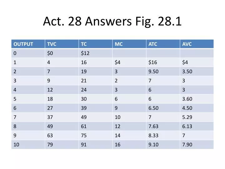
Act. 28 Answers Fig. 28.1. Fig. 28.2. Fig. 28.2. (C) How would you interpret the vertical distance between the average total cost and average variable cost curves? It is average fixed cost (AFC). As AFC decreases continuously, the ATC and the AVC curves get closer together. Fig. 28.2.

E N D
Fig. 28.2 • (C) How would you interpret the vertical distance between the average total cost and average variable cost curves? It is average fixed cost (AFC). As AFC decreases continuously, the ATC and the AVC curves get closer together.
Fig. 28.2 • (D)Why does average total cost decline at first, then start rising as output is increased? When MC < ATC, ATC declines. When MC > ATC, ATC rises. Why does MC rise? Diminishing MPP
Fig. 28.2 • (E) The marginal cost curve intersects both average cost curves (ATC and AVC) at their minimum points. Why? If the marginal is below the average, the average is decreasing. If the marginal is above the average, the average is increasing. Therefore, the average crosses the marginal at the average’s lowest point.
Fig. 28.2 • (F) If fixed costs were $20 instead of $12, how would the change affect average variable costs and marginal costs? They would not change. (But ATC would increase.) Fixed cost, by definition, does not change when output changes. Therefore, fixed cost has no influence on variable cost or marginal cost.
Fig. 28.2 • #2 • (A) Draw and label the average and marginal revenue curves on your graph. A horizontal line at $11.00
Fig. 28.2 • (B) In order to maximize profits, Fiasco would sell 7 units, at a price of $11.00 . Its average total cost would be $7.00 . Its average revenue would be $11.00 . It would earn a per unit profit of $4.00 and total profit of $28.00 ($4 x 7) per day.
Fig. 28.2 • (C) If the firm produced instead at the quantity that minimized its average total cost, it could sell 4.5 units, at a price of $11.00 . Its average total cost would be $6.00 (or less than $6.00, say, $5.50). If the market price were $11, its average revenue would be $11.00 . It would earn a per-unit profit of $5.50 and total profit of $24.75 ($5.50 x 4.5) per day.
Fig. 28.2 • (D) If the competitive market price fell to $5 a unit, Fiasco would sell 4 units. Average total cost would be $6.00 . It would earn a per-unit (profit / loss) of $1.00 and a total (profit / loss) of $4.00 ($1.00 x 4) per day.
Fig. 28.3 Part B • (B) The level of output at which average total cost is at a minimum is between 3 and 4 units. • At this output, average total cost is $6.00 .
Figure 28.4Price and Quantity Supplied • (D) In general, the supply schedule (curve) of a perfectly competitive firm coincides with its MC schedule (curve) in the range where MC is greater than AVC .
Figure 28.5 • (A) Fill in the industry supply schedule in Figure 28.5. Then answer the following questions by filling in the answer blanks, underlining the correct words in parentheses or writing a sentence. • (B) Explain briefly how the short-run supply schedule (curve) of a competitive industry is derived. The horizontal sum at each price of all firms’ supply curves = MC above minimum AVC.
Figure 28.5 • (C) Given the present 1,000 firms in the industry, the present market price is $8.00 ; the present equilibrium quantity is 6,000 units. At this price, each firm will be making ( positive economic profit / zero economic profit / negative economic profit / economic losses).
Figure 28.5 • (D) Given the equilibrium above, and assuming that other firms can enter the industry with the same cost as the present firms, the number of firms in the industry in the long run will tend to ( increase / decrease/ remain constant) and the price will tend to (increase / decrease / remain constant). The output of the industry will tend to ( increase / decrease / remain constant), while output per firm will (increase / decrease / remain constant).
Figure 28.5 • (E) If this is a constant-cost industry (i.e., costs per unit of output are constant as the industry expands), the long-run equilibrium price for the industry will be $6.00 ; output per firm will be 4 units. There will be 2,000 firms in the industry, each earning 0 economic profits; industry output will be 8,000 units. The equilibrium price coincides with the minimum per-unit cost of production. Emphasize minimum ATC
Figure 28.5 • (F) Can you see why, under the conditions described above, that the long-run market-supply curve for this industry would appear as a horizontal line on a graph? Explain. Other firms can enter and eliminate any economic profit that appears. Thus, in the long run, all firms will be at minimum ATC.
Figure 28.5 • (G) Using the cost curves in Figure 28.2, at what price would this long-run horizontal line be plotted? $6.00 Explain why it would be at this price. This is the quantity where MC equals ATC at the minimum level of ATC. The perfectly competitive firm breaks even in the long run at minimum ATC: its most technically efficient point.