Download
1 / 21
210 likes | 212 Views
This paper discusses the design goals, structure, and application of a coupled ocean-atmosphere model using horizontally icosahedral and vertically hybrid-isentropic/isopycnic grids. The model aims to achieve a global domain, no grid mismatch at the ocean-atmosphere interface, and similar intrinsic model climate and variability to observed data. It is important for reducing biases in simulations ranging from 1 day to 1 month, and focuses on key indicators such as ENSO, MJO, wintertime stratospheric warming, and tropospheric blocking frequency.

E N D
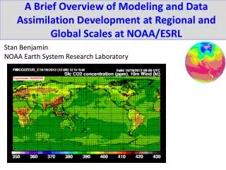
Coupled ocean-atmosphere modeling on horizontally icosahedral and vertically hybrid-isentropic/isopycnic grids Rainer Bleck, Shan Sun, Haiqin Li, Stan Benjamin NOAA Earth System Research Laboratory Boulder, Colorado April 2016
Design goals:(some reached, some pending) • Global domain • No grid mismatch at ocean-atmointerface • Same horizontal resolution as medium-range NWP models (=> eddy-permitting ocean) • Envisioned forecast time range: 1 day - 1 month • Intrinsic model climate & variability similar to observed • Deemed important for reducing biases even in simulations as short as 1 month. • Key variability indicators: ENSO, MJO, wintertime stratospheric warming, tropospheric blocking freq. • Steadiness of meridional overturning circulations (Hadley, Brewer-Dobson, thermohaline circ.)
The coupled model • Atmosphere:FIM (F=flow-following, I=icosahedral) • Horizontal grid: icosahedral; resolution choices 240, 120, 60, 30, 15 km (104 - 2.5x10⁶ grid cells) • Vertical grid: isentropicaloft, reverting to terrain-following near the ground. Adaptive, 64 layers. • Ocean:i-HYCOM (icosahedral version of Hybrid Coordinate Ocean Model) • Horizontal grid: same as atmosphere • Vertical grid: isopycnicat depth, reverting to p near the sea surface. Adaptive, 32 layers. • Flux Coupler: a non-issue (matching grid cells!) • important: no coastline ambiguities • Atmosphere in charge of computing surface fluxes • No flux adjustment or post-mortem bias removal
Additional model details -- atmosphere • Designed and used at NOAA-ESRL as medium-range NWP model (http://fim.noaa.gov) • Hydrostatic. • Arakawa-A grid (all variables carried in grid cell center). • Finite-volume numerics (2nd order). • Column physics imported from GFS (NOAA-NCEP). • Rudimentary river-routing scheme • Essential for closing freshwater cycle (=> ocean salinity). • Indirect addressing (table lookup) for lateral neighbor interactions. Efficiently parallelized.
Additional model details -- ocean • Essentially HYCOM, but rewritten for icosahedral mesh. • Vertical coordinate: potential density (rpot) • referenced to 1km depth. • drpot/dt=0 in adiab.flow (i.e. incompressible w.r.t. rpot) • Prognostic variables: T, S, u, v, dp (layer thickness). • Basic 1-layer ice model, free drift. • Simplified barotropic-baroclinic mode splitting • 3D equations for u,v,dpsolved on “barotropic” time steps. • Bonus: no need to express freshwater fluxes as virtual salt fluxes. • Software engineering innovations (parallelization etc.) inherited from FIM. • Tightly coupled to atmosphere on “baroclinic” time steps.
1. Short-range application: Hurricane • Chosen example: Hurricane Sandy, October 2012 • Initial state (ocean and atmosphere) from NOAA-NCEP Climate Forecast System v.2 • Model resolution ~15km. • Ocean is eddy-permitting, but no realistic eddies in initial state.
Sample results Hurricane Sandy 1 triangle=0.5Pa 1 triangle=25cm/s Wind stress (left) and surface currents (right) off the U.S. east coast in 5.5 day forecast starting at 12GMT, 23 Oct 2012. Note: ocean response dominated by inertial waves. No hurricane-induced vortex.
Sample results Surface temperature (left) and salinity (right) in 5.5 day forecast starting at 12GMT, 23 Oct 2012. Note: SST appears to be mainly controlled by cloudiness/precip, not wind stress.
1st layer thickness: 2m Zonal vertical section at 370N showing temperature and coordinate layer interfaces. Top section is blowup of bottom section. Note shallowness of srfc. cold layer. Gulf Stream front
2. Medium-range application: Does intrinsic model variability change over time?
Frequency of blocking episodes (Pelly-Hoskins) in 600 30-day coupled simulations spread over years 1999-2010. Mesh size 30km
3. Long-range application: Does the model support the leading coupled mode in the ocean-atmosphere system?
Top: Nino3 index from final 50-yr period of coupled simulations. Mesh size 120km. Bottom: observed index. Grell-Freitas cloud parameterization: mod 2 Grell-Freitas cloud parameterization: mod 3
Does the model maintain a reasonably steady Atlantic meridional overturning circulation?
Time series of oceanic mass flux (Atlantic overturning, Drake Passage, Lombok Strait) in multi-decadal coupled simulation. Mesh size 120km. Note low AMOC (25% of observed strength) Units: 1 Sverdrup = 106m3/s
low/high vertical diffusivity Which component of the coupled model is responsible for the low AMOC? Shown here are two ocean-only simulations, forced by observed atmosphere (CORE-II). AMOC is acceptable in this case.
Salinity trends in “concentration basins”result from precip/evaporation imbalances. Are they tolerable?
Sea surface temperature in concentration basins Year 0 Year 10 Year 20
Sea surface salinity in concentration basins Year 0 Year 10 Year 20 Capping of salinity required here, other basins OK.
Conclusions and Outlook • Converting a weather model into a GCM is a challenge, especially when coupling it to an ocean • Surface fluxes “thrown away” in atmo-only applications suddenly become important • Column physics codes written for NWP are not necessarily conservative (energy, freshwater cycle) • Convective cloud parameterization requires intensive tuning to achieve zero net radiation balance • Simulation of ENSO variability moderately successful. • Subtle decrease in blocking frequency with forecast duration on monthly time scale. • Model maintains weak AMOC on decadal time scales. • By using a unique combination of nonstandard 3D grids (icosahedral + isentropic/isopycnic) we strive to contribute to the genetic diversity in coupled multi-model ensemble applications.