Download
1 / 23
310 likes | 742 Views
Harmonic Analysis. The observed flow u’ may be represented as the sum of M harmonics: u’ = u 0 + Σ j M =1 A j sin ( j t + j ). For M = 1 harmonic (e.g. a diurnal or semidiurnal constituent): u’ = u 0 + A 1 sin ( 1 t + 1 ). With the trigonometric identity:

E N D
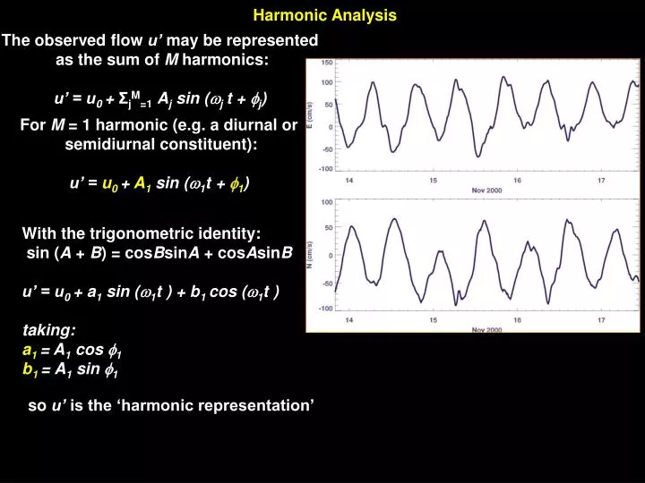
Harmonic Analysis The observed flow u’ may be represented as the sum of M harmonics: u’ = u0 + ΣjM=1Aj sin (j t + j) For M = 1 harmonic (e.g. a diurnal or semidiurnal constituent): u’ = u0+ A1 sin (1t + 1) With the trigonometric identity: sin (A + B) = cosBsinA + cosAsinB u’ = u0 + a1 sin (1t ) + b1 cos (1t ) taking: a1= A1 cos 1 b1= A1 sin 1 so u’ is the ‘harmonic representation’
Using u’ = u0 + a1 sin (1t ) + b1 cos (1t ) Then: 2 = ΣN {u 2 - 2uu0 - 2ua1 sin (1t ) - 2ub1 cos (1t ) + u02 + 2u0a1 sin (1t ) + 2u0b1 cos (1t ) + 2a1 b1 sin (1t ) cos (1t ) + a12sin2 (1t ) + b12cos2 (1t ) } The squared errors between the observed current u and the harmonic representation may be expressed as 2 : 2 = ΣN [u - u’ ]2 = u 2 - 2uu’ + u’ 2 Then, to find the minimum distance between observed and theoretical values we need to minimize 2 with respect to u0 a1and b1, i.e., δ 2/ δu0 , δ 2/ δa1 , δ 2/ δb1 : δ2/ δu0 = ΣN {-2u +2u0 + 2a1 sin (1t ) + 2b1 cos (1t ) } = 0 δ2/ δa1 = ΣN { -2u sin (1t ) +2u0 sin (1t ) + 2b1 sin (1t ) cos (1t ) + 2a1 sin2(1t ) } = 0 δ2/ δb1 = ΣN {-2u cos (1t ) +2u0 cos (1t ) + 2a1 sin (1t ) cos (1t ) + 2b1 cos2(1t ) } = 0
ΣN { u = u0 + a1 sin (1t ) + b1 cos (1t ) } ΣN { u sin (1t ) = u0 sin (1t ) + b1 sin (1t ) cos (1t ) + a1 sin2(1t ) } ΣN { u cos (1t ) = u0 cos (1t ) + a1 sin (1t ) cos (1t ) + b1 cos2(1t ) } ΣN u N ΣN sin (1t ) ΣN cos (1t ) u0 ΣN {-2u +2u0 + 2a1 sin (1t ) + 2b1 cos (1t ) } = 0 ΣN u sin (1t ) = ΣN sin (1t ) ΣN sin2(1t ) ΣN sin (1t ) cos (1t ) a1 ΣN u cos (1t ) ΣN cos (1t ) ΣN sin (1t ) cos (1t ) ΣN cos2(1t ) b1 ΣN {-2u sin (1t ) +2u0 sin (1t ) + 2b1 sin (1t ) cos (1t ) + 2a1 sin2(1t ) } = 0 ΣN { -2u cos (1t ) +2u0 cos (1t ) + 2a1 sin (1t ) cos (1t ) + 2b1 cos2(1t ) } = 0 X = A-1 B Rearranging: And in matrix form: B = A X
Finally... The residual or mean is u0 The phase of constituent 1 is: 1 = atan( b1 / a1 ) The amplitude of constituent 1 is: A1 = ( b12+ a12 )½ Pay attention to the arc tangent function used. For example, in IDL you should use atan (b1,a1) and in MATLAB, you should use atan2
Matrix A is then: N ΣN sin (1t ) ΣN cos (1t ) ΣN sin (2t ) ΣN cos (2t ) ΣN sin (1t ) ΣN sin2(1t ) ΣN sin (1t ) cos (1t ) ΣN sin (1t ) sin (2t ) ΣN sin (1t ) cos (2t ) ΣN cos (1t ) ΣN sin (1t ) cos (1t ) ΣN cos2(1t ) ΣN cos (1t ) sin (2t ) ΣN cos (1t ) cos (2t ) ΣN sin (2t ) ΣN sin (1t ) sin (2t ) ΣN cos (1t ) sin (2t ) ΣN sin2(2t ) ΣN sin (2t ) cos (2t ) ΣN cos (2t ) ΣN sin (1t ) cos (2t ) ΣN cos (1t ) cos (2t ) ΣN sin (2t ) cos (2t ) ΣN cos2 (2t ) Remember that: X = A-1 B and B = u0 a1 b1 a2 b2 ΣN u ΣN u sin (1t ) X = ΣN u cos (1t ) ΣN u sin (2t ) ΣN u cos (2t ) For M = 2 harmonics (e.g. diurnal and semidiurnal constituents): u’ = u0+ A1 sin (1t + 1) + A2 sin (2t + 2)
Goodness of Fit: Σ [< uobs > - upred] 2 ------------------------------------- Σ [<uobs > - uobs] 2 Root mean square error: [1/N Σ (uobs - upred) 2] ½
Fit with M2, S2, K1 Rayleigh Criterion: record frequency ≤ ω1 – ω2
Fit with M2, S2, K1, M4, M6
Tidal Ellipse Parameters M2 S2 K1 Major axis: M minor axis: m ellipticity = m/ M Phase Orientation
Tidal Ellipse Parameters amplitude of the counter-clockwise rotary component phase of the clockwise rotary component phase of the counter-clockwise rotary component Ellipse Coordinates: ua, va, up, vpare the amplitudes and phases of the east-west and north-south components of velocity amplitude of the clockwise rotary component The characteristics of the tidal ellipses are: Major axis = M = Qcc + Qc minor axis = m = Qcc - Qc ellipticity = m / M Phase = -0.5 (thetacc - thetac) Orientation = 0.5 (thetacc + thetac)
M2 S2 K1
Complex Demodulation Time series X(t)taken as nearly periodic plus non-periodic Z(t), still varying in time. Amplitude A and phase ϕof the nearly periodic signal are allowed to be time-dependent but vary slowly compared to the frequency ω. X(t) = A(t) cos(ωt +ϕ(t))+ Z(t) Demodulate by multiplying times Low-pass filter to remove frequencies at or above Varies slowly, independent of Varies at frequency 2 Varies at frequency
Amplitude of complex demodulated series at semidiurnal frequency Ensenada de La Paz, Mexico
YAVAROS BAY, MEXICO Dworak, J. A., and J. Gomez-Valdes (2005), J. Geophys. Res., 110, C01007, doi:10.1029/2003JC001865.
Station M Dworak, J. A., and J. Gomez-Valdes (2005), J. Geophys. Res., 110, C01007, doi:10.1029/2003JC001865.
Puerto Morelos Coral Reef Lagoon Puerto Morelos Lagoon North America Atlantic Ocean Northern Inlet Gulf of Mexico Pargos Spring Mexico Caribbean Sea Yucatan Peninsula Central Inlet Pacific Ocean Coronado et al. 2007 Southern Inlet Sabrina Parra