Download
1 / 31
310 likes | 493 Views
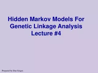
Genetic Linkage Analysis using HMMs Lecture 7. Prepared by Dan Geiger.

E N D
Genetic Linkage Analysis using HMMsLecture 7 . Prepared by Dan Geiger
Part I: Quick look on relevant geneticsPart II: The use of HMMs Part III: Case study: Werner’s syndrome Gene Hunting: find genes responsible for a given diseaseMain idea: If a disease is statistically linked with a marker on a chromosome, then tentatively infer that a gene causing the disease is located near that marker. Outline
Chromosome Logical Structure Locus – the location of markers on the chromosome. Allele – one variant form (or state) of a gene/marker at a particular locus. By markers we mean genes, Single Nucleotide Polymorphisms, Tandem repeats, etc. Locus1 Possible Alleles: A1,A2 Locus2 Possible Alleles: B1,B2,B3
Phenotype versus Genotype • The ABO locus determines detectable antigens on the surface of red blood cells. • The 3 major alleles (A,B,O) determine the various ABO blood types. • O is recessive to A and B. A and B are dominant over O. Alleles A and B are codominant. Note: genotypes are unordered.
Recombination Phenomenon Male or female A recombination between 2 genes occurred if the haplotype of the individual contains 2 alleles that resided in different haplotypes in the individual's parent. (Haplotype – the alleles at different loci that are received by an individual from one parent). תאי מין: ביצית, או זרע
Homolog chromosomes showing Chaismata כרומוזומים הומולוגיים המראים כיאסמתה Sister chromatids הכיאסמה היא הביטוי הציטולוגי לשחלוף. Chaisma(ta) is the cellular expression of recombination.
O A2/A2 A A1/A1 1 2 A A2/A2 A A1/A2 3 4 A | O A2 | A2 A O A1 A2 O O A2 A2 O O A1 A2 Recombinant O A1/A2 5 Example: ABO and the AK1 marker on Chromosome 9 Phase inferred Recombination fraction = 16/100. One centi-morgan means one recombination every 100 meiosis. In our case it is 16cM. One centi-morgan corresponds to approx 1M nucleotides (with large variance) depending on location and sex.
D A2/A2 H A1/A1 1 2 H A2/A2 H A1/A2 3 4 H | D A2 | A2 H D A1 A2 D D A2 A2 D D A1 A2 Recombinant D A1/A2 5 Example for Finding Disease Genes Phase inferred We use a marker with codominant alleles A1/A2. We speculate a locus with alleles H (Healthy) / D (affected) If the expected number of recombinants is low (close to zero), then the speculated locus and the marker are tentatively physically closed.
H A2/A2 H A1/A1 Phase ??? 1 2 H A2/A2 H A1/A2 3 4 Possible Recombinant D D A1 A2 H D A1 A2 H | D A2 | A2 D A1/A2 5 Recombination cannot be simply counted One can compute the probability that a recombination occurred and use this number as if this is the real count.
Comments about the example Often: • Pedigrees are larger and more complex. • Not every individual is typed. • Recombinants cannot always be determined. • There are more markers and they are polymorphic (have more than two alleles).
Genetic Linkage Analysis • The method just described is called genetic linkage analysis. It uses the phenomena of recombination in families of affected individuals to locate the vicinity of a disease gene. • Recombination fraction is measured in centi morgans and can change between males and females. • Next step: Once a suspected area is found, further studies check the 20-50 candidate genes in that area.
Using the Maximum Likelihood Approach The probability of pedigree data Pr(data | ) is a function of the known and unknown recombination fractions (the unknown is denoted by ). How can we construct this likelihood function ? The maximum likelihood approach is to seek the value of which maximizes the likelihood function Pr(data | ) . This is the ML estimate.
Constructing the Likelihood function First, we determine the variables describing the problem. Lijm = Maternal allele at locus i of person j. The values of this variables are the possible alleles li at locus i. Lijf = Paternal allele at locus i of person j. The values of this variables are the possible alleles li at locus i (Same as for Lijm) . Xij= Unordered allele pair at locus i of person j. The values are pairs of ith-locus alleles (li,l’i). “The genotype” Yj= person j is affected/not affected. “The phenotype”. Sijm= a binary variable {0,1} that determines which maternal allele is received from the mother. Similarly, Sijf= a binary variable {0,1} that determines which paternal allele is received from the father. It remains to specify the joint distribution that governs these variables. HMMs turn to be a reasonable choice.
Si3f Li2f y2 Xi2 Li2m Li3f Xi3 Li3m Y3 Li1f Xi1 Y1 Li1m Si3m Locus 2 (Disease) Locus 3 Locus 4 Locus 1 The model This model depicts the qualitative relations between the variables. We will now specify the joint distribution over these variables.
L11m L11f L12m L12f X11 S13m X12 S13f L13f L13m X13 Probabilistic Model for Recombination L21m L21f L22m L22f X21 S23m X22 S23f Y2 Y1 L23f L23m X23 Y3 is the recombination fraction between loci 2 & 1.
Li1f Li1m Xi1 Si3m Y1 Li3m Details regarding the Loci P(L11m=a) is the frequency of allele a. X11 is an unordered allele pair at locus 1 of person 1 = “the data”. P(x11 | l11m, l11f) = 0 or 1 depending on consistency The phenotype variables Yj are 0 or 1 (e.g, affected or not affected) are connected to the Xij variables (only in the disease locus). For example, model of perfect recessive disease yields the penetrance probabilities: P(y11 = sick | X11= (a,a)) = 1 P(y11 = sick | X11= (A,a)) = 0 P(y11 = sick | X11= (A,A)) = 0
X1 X1 X2 X2 X3 X3 Xi-1 Xi-1 Xi Xi Xi+1 Xi+1 Hidden Markov Model In our case S1 S2 S3 Si-1 Si Si+1 X1 X2 X3 Yi-1 Xi Xi+1 The compounded variable Si = (Si,1,m,…,Si,n,f)is called the inheritance vector. It has 22n states where n is the number of persons that have parents in the pedigree (non-founders). The compounded variable Xi = (Xi,1,…,Xi,n) is the data regarding locus i. Similarly for the disease locus we use Yi. To specify the HMM we now explicate the transition matrices from Si-1 to Si and the matrices P(xi|Si).
00 01 10 11 00 01 10 11 The transition matrix Recall that we wrote: All i are usually known except the one before the disease locus . Extending this matrix to the smallest inheritance vector (n=1), we get: Let d=hamming distance between state si-1 and state si. Then the transition probability is given by id(1-i)2n-d
L21m L21f L22m L22f X21 S23m X22 S23f = P(l21m)P(l21f)P(l22m)P(l22f) P(x21 | l21m, l21f) P(x22 | l22m, l22f) P(x23 | l23m, l23f) P(l23m | l21m, l21f, S23m) P(l23f | l22m, l22f, S23f) L23f L23m l21m,l21f,l22m,l22f l22m,l22f X23 Model for locus 2 Probability of data in one locus given the inheritance vector (emission probabilities) P(x21, x22 , x23 |s23m,s23f) = The five last terms are always zero-or-one, namely, indicator functions.
Probability of data in the disease locus given the inheritance vector (emission probabilities) P(y1, y2 , y3 |s23m,s23f) = = P(l21m) P(l21f) P(l22m) P(l22f) P(x21 | l21m, l21f) P(x22 | l22m, l22f) P(x23 | l23m, l23f) P(l23m | l21m, l21f, S23m) P(l23f | l22m, l22f, S23f) l21m,l21f,l22m,l22f l22m,l22f ,x21,x22,x23 P(y1|x21) P(y2|x22) P(y3|x23)
S1 X1 S2 X3 Xi Si Slast X1 X1 X3 X2 Xi Xi Xlast S Xi-1 Xi-1 Y Finding the best location
S1 X1 X3 S2 Si Xi Slast X1 X1 X3 X2 Xi Xi Xlast Xi-1 S Xi-1 Y Finding the best location Simplest algorithm: For each possible locations on the genetic map, place the disease locus, say in the middle, and compute using the forward algorithm, the probability of data given that location. Data here means one assignment for the Xi variables and for Y. Choose the maximum of all options.
S1 X1 S2 X3 Si Xi Slast X1 X1 X3 X2 Xi Xi Xlast Xi-1 S Xi-1 Y Finding the best location Second algorithm: Run the forward-backward algorithm and store intermediate results. Use these to compute probability of data at each location, all at once. Choose the maximum of all options. At each segment one can try several values for and choose the best. Or use EM to learn the best value.
Part III: Case study Werner’s Syndrome A successful application of genetic linkage analysis using HMM software (GeneHunter)
The Disease • First references in 1960s • Causes premature ageing • Autosomal recessive • Linkage studies from 1992 • WRN gene cloned in 1996 • Subsequent discovery of mechanisms involved in wild-type and mutant proteins
One Pedigree’s Data (out of 14) Pedigree number Father’s ID Sex: 1=male 2=female Unknown marker alleles 1 115 0 0 2 1 0 1 0 1 2 1 2 3 3 1 2 1 1 1 3 2 2 1 0 0 1 0 1 0 1 0 1 126 0 0 1 1 0 0 1 0 1 2 1 2 3 3 1 2 1 1 1 3 2 2 1 0 0 1 0 1 1 0 1 111 0 0 1 1 0 1 0 1 2 0 2 0 3 1 2 1 1 1 3 1 2 1 0 0 1 0 1 0 0 0 1 122 111 115 2 1 0 0 0 0 0 0 0 0 0 0 0 0 0 0 0 0 0 0 0 0 0 0 0 0 0 0 1 125 0 0 2 1 0 0 0 0 0 0 0 0 0 0 0 0 0 0 0 0 0 0 0 0 0 0 0 0 0 0 1 121 111 115 1 1 2 0 1 2 1 2 3 3 1 2 1 1 1 3 2 2 1 0 0 1 0 1 0 1 0 1 1 135 126 122 2 1 0 0 0 0 0 0 0 0 0 0 0 0 0 0 0 0 0 0 0 0 0 0 0 0 0 0 1 131 121 125 1 1 0 0 0 0 0 0 0 0 0 0 0 0 0 0 0 0 0 0 0 0 0 0 0 0 0 0 1 141 131 135 2 2 1 2 1 1 1 1 1 1 1 1 1 1 1 1 1 1 1 1 1 1 1 1 1 1 1 1 Known marker alleles Individual ID Mother’s ID Status: 1=healthy 2=diseased
Marker File Input 1 disease locus + 13 markers 14 0 0 5 0 0.0 0.0 0 1 2 3 4 5 6 7 8 9 10 11 12 13 14 1 2 0.995 0.005 1 0 0 1 3 6# D8S133 0.0200 0.3700 0.4050 0.0050 0.0500 0.0750 ...[other 12 markers skipped]... 0 0 10 7.6 7.4 0.9 6.7 1.6 2.5 2.8 2.1 2.8 11.4 1 43.8 1 0.1 0.45 Recessive disease requires 2 mutant genes First marker has 6 alleles First marker’s name Recombination distances between markers First marker founder allele frequencies
Genehunter Output position LOD_score information 0.00 -1.254417 0.224384 1.52 2.836135 0.226379 ...[other data skipped]... 18.58 13.688599 0.384088 19.92 14.238474 0.401992 21.26 14.718037 0.426818 22.60 15.159389 0.462284 22.92 15.056713 0.462510 23.24 14.928614 0.463208 23.56 14.754848 0.464387 ...[other data skipped]... 81.84 1.939215 0.059748 90.60 -11.930449 0.087869 Putative distance of disease gene from first marker in recombination units Log likelihood of placing disease gene at distance, relative to it being unlinked. Most ‘likely’ position Maximum log likelihood score
Marker Inter- Distance distance from first DHS133 0.0 D8S136 7.6 7.6 D8S137 7.4 15.0 D8S131 0.9 15.9 D8S339 6.7 22.6 D8S259 1.6 24.2 FGFR 2.5 26.7 D8S255 2.8 29.5 ANK 2.1 31.6 PLAT 2.8 34.4 D8S165 11.4 45.8 D8S166 1.0 46.8 D8S164 43.8 90.6 Locating the Marker
Final Location Marker D8S259 location of marker D8S339 Marker D8S131 WRN Gene final location Error in location by genetic linkage of about 1.25M base pairs.