Download
1 / 77
770 likes | 893 Views
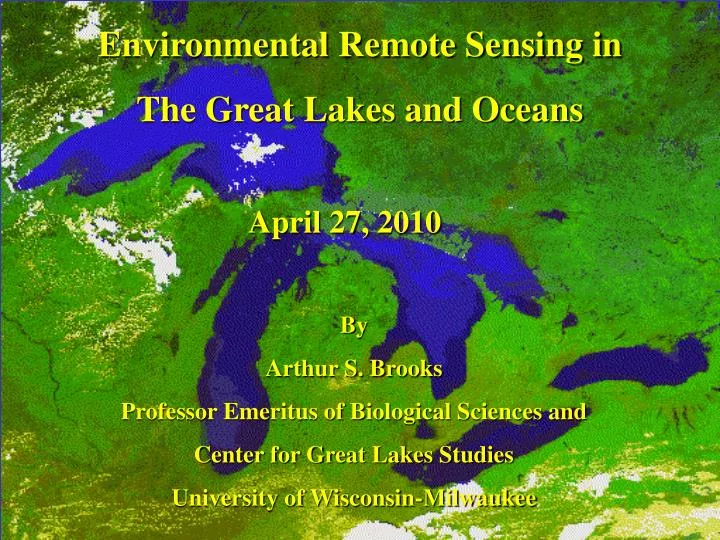
Environmental Remote Sensing in The Great Lakes and Oceans. April 27, 2010. By Arthur S. Brooks Professor Emeritus of Biological Sciences and Center for Great Lakes Studies University of Wisconsin-Milwaukee. EARTH: THE WATER PLANET. EARTH: THE WATER PLANET.

E N D
Environmental Remote Sensing in The Great Lakes and Oceans April 27, 2010 By Arthur S. Brooks Professor Emeritus of Biological Sciences and Center for Great Lakes Studies University of Wisconsin-Milwaukee
WHERE IS ALL THE WATER TODAY ?? • THE OCEANS 1,348 M km3
WHERE IS ALL THE WATER TODAY ?? • THE OCEANS 1,348 M km3 • ICE CAPS & GLACIERS 29 M km3
WHERE IS ALL THE WATER TODAY ?? • THE OCEANS 1,348 M km3 • ICE CAPS & GLACIERS 29 M km3 • GROUNDWATER 8.0 M km3
WHERE IS ALL THE WATER TODAY ?? • THE OCEANS 1,348 M km3 • ICE CAPS & GLACIERS 29 M km3 • GROUNDWATER 8.0 M km3 • THE ATMOSPHERE 0.5 M km3
WHERE IS ALL THE WATER TODAY ?? • THE OCEANS 1,348 M km3 • ICE CAPS & GLACIERS 29 M km3 • GROUNDWATER 8.0 M km3 • THE ATMOSPHERE 0.5 M km3 • SURFACE FRESHWATER 0.2 M km3
ALL IN ONE LITER (1000 ml) • 974.7 ml (97.5%) SALTWATER • 25.3 ml (2.5%) FRESH WATER
ALL FRESHWATER (25.3 ml) • 17.6 ml ICE CAPS AND GLACIERS • 7.6 ml GROUNDWATER • 0.1 ml SURFACE WATER(2 drops)
SURFACE FRESHWATER0.1 ml(2 DROPS) • 0.02 ml (20%) LAKE BAIKAL (RUSSIA) • 0.02 ml (20%) OUR GREAT LAKES • 0.06 ml (60%) ALL OTHER RIVERS AND LAKES
The Coastal Zone Color Scanner (CZCS) is a sensor specifically developed to study ocean color properties. These properties can be related to organic content, such as plankton, as well as sediment. CZCS launched in October 1978, as part of Nimbus-7's instrument complement and continued to operate until late 1986. It sensed colors in the visible region in four bands, each 0.02 µm in bandwidth, centered at 0.44 (1), 0.52 (2), 0.57 (3), and 0.67 (4) µm. A fifth band between 0.7 and 0.8 µm monitored surface vegetation and band six, at 10.5-12.5 µm sensed sea surface temperatures. Here is the first CZCS before fitting onto the Nimbus spacecraft:
CZCS distribution of chlorophyll on a global scale averaged between 1978 and 1986
Moderate-resolution Imaging Spectroradiometer (MODIS) -integrated on the Terra (EOS AM-1) and Aqua (EOS PM-1) spacecraft
MODIS, for Moderate (resolution) Imaging Spectrometer, covers usually large areas, such as the Black Sea shown here:
A recent image from Terra's MODIS, using bands at 11 and 12 µm, shows how sharp the temperature contrast can be between the main Gulf stream (red) and surrounding waters:
Another MODIS image of the warm Gulf Stream emphasizes its tendency to meander as it moves northward:
In the color coding, blues correspond to the lowest levels of phytoplankton and reds to the highest. Note the eddies or rings. Phytoplankton tends to concentrate along the edges of warm core rings (which rotate clockwise) but concentrate centrally in cold core rings (counterclockwise motion).
The MODIS instrument on Aqua picked out a large phytoplankton bloom off the northern coast of Norway on July 19, 2003. Most of the blue-green color in the (near true color) image below was found to be due to plankton whose shells) are composed of chalky Calcium carbonate (CaCO3.)
SeaWiFS(Sea-viewing Wide Field-of-View Sensor), launched on August 1, 1997. The sensor system monitors ocean color variations, especially those caused by concentrations of plankton and other sea life. Thus, the prime objectives are: 1) to quantify ocean plankton production; 2) to determine observable couplings of physical/biological processes; and 3) to characterize estuarine and coastal ecosystems. The SeaWiFS sensor consists of eight channels at: 412, 443, 490, 510, 555, 670, 765, and 865 nm, each with bandwidths of 20 or 40 nm. From an orbital altitude of 705 km, spatial resolution is about 1.1 km.
On SeaWiFS, several bands cover the blue, green, and red parts of the visible spectrum, and into the near infrared, yielding data that can be used to display variations in ocean color or, for particular bands, indications of the distribution and intensity of chlorophyll that resides mainly in surficial plankton. This SeaWiFS image maps the generalized ocean colors as well as chlorphyll concentrations (in red, yellow, and orange colors) on a near global scale during September, 1997. On SeaWiFS, several bands cover the blue, green, and red parts of the visible spectrum, and into the near infrared, yielding data that can be used to display variations in ocean color or, for particular bands, indications of the distribution and intensity of chlorophyll that resides mainly in surficial plankton. This SeaWiFS image maps the generalized ocean colors as well as chlorphyll concentrations (in red, yellow, and orange colors) on a near global scale.
SeaWiFS produces regional scale images in which eddies and circulation patterns are evident. In this view of western North America, marine eddies have formed off the British Columbia coast around Queen Charlotte; to the west is another eddy-like pattern made by clouds.
Red Tide occurred north of the Florida Keys in 2002, as seen in this SeaWiFs image that renders the red algae in almost natural color; Key West
In Situ Validation Data • TERRA and AQUA SST and SST4 products show similar behavior with respect to in situ retrievals to date Right - Explorer cruise tracks that provide bias reference using M-AERI observations Lower Left - Drifting buoys, used to compute SST equation retrieval coefficients Lower Right - Global M-AERI cruise tracks, final validation suite Drifting Buoys
Dec 10 2000 SeaWiFS - MODIS Chlorophyll Comparisons SeaWiFS Chlorophyll a MODIS Chlorophyll a J. Campbell et al.
SCIENCE QUESTIONS (Ocean NPP) • This Product Derives Ocean Net Primary Production and Annual Export Production from Chlorophyll, Light (PAR), SST, and Mixed Layer Depth • Carbon fixed/m2/day - Needed to understand: • Magnitude and Variability of ONPP, and uncertainties. • Ecosystem dynamics (coupling with physical forcings) • Food chain effects (fisheries resources) • Carbon cycle (carbon export, pCO2 and hence air sea C flux) • RELEVANT SCIENCE QUESTIONS for ONPP • Variability - How are global ecosystems changing? • Response - How do ecosystems respond to and affect global environmental change and the carbon cycle?
Chlor_MODIS (Clark) Chlorophyll-a (empirical) December, 2000 Chlor_a_2 Chlorophyll-a (SeaWiFS analog) OC3M OReilly et al Chlor_a_3 (Carder) Chlorophyll-a (semi-analytic) Input for ONPP, Fluorescence Efficiency .01 0.1 1.0 10. 20. Chlorophyll a (mg m-3)
Weekly PAR December 10, 2000 Derived from GSFC Data Assimilation Office GEOS 3.2.5 3 hr retrievals.
MODIS SST December 10, 2000 MODIS Daytime 11-12 mm SST D1 Also used for Chlorophyll nut depletion Temp.
Mixed Layer Depth Dec. 10, 2000 Mixed Layer Depth is averaged from daily values retreived by Fleet Numerical Monterey Oceanographic Center’s (FNMOC) OTIS model, obtained through NOAA-Navy net by GES DAAC.
P1 Behrenfeld- Falkowski P2 Howard Yoder Ryan Dec 10-18,2000 3.3.1
Name the Great Lakes ? Huron
Name the Great Lakes ? Huron Ontario
Name the Great Lakes ? Huron Ontario Michigan
Name the Great Lakes ? Huron Ontario Erie Michigan
Name the Great Lakes ? Superior Huron Ontario Erie Michigan