Download
1 / 23
230 likes | 299 Views
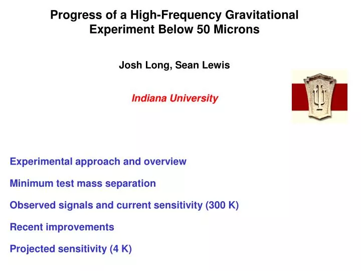
Progress of a High-Frequency Gravitational Experiment Below 50 Microns. Josh Long, Sean Lewis. Indiana University. Experimental approach and overview. Minimum test mass separation. Observed signals and current sensitivity (300 K). Recent improvements. Projected sensitivity (4 K).

E N D
Progress of a High-Frequency Gravitational Experiment Below 50 Microns Josh Long, Sean Lewis Indiana University Experimental approach and overview Minimum test mass separation Observed signals and current sensitivity (300 K) Recent improvements Projected sensitivity (4 K)
Experimental Approach Planar Geometry Resonant detector with source mass driven on resonance 1 kHz operational frequency - simple, stiff vibration isolation Double-rectangular torsional detector: high Q, low thermal noise Stiff conducting shield for background suppression ~ 5 cm Source and Detector Oscillators Shield for Background Suppression
Central Apparatus Scale: 1 cm3 “Taber” vibration isolation stacks: Brass disks hanging from fine wires; make set of soft springs which attenuate at ~1010 at 1 kHz vibration isolation stacks tilt stage Installed in 75 liter vacuum bell jar (10-7 torr) for further suppression of acoustic forces transducer amp box detector mass shield READOUT source mass PZT bimorph Capacitive probe above large detector rectangle connects to JFET, Lock-in amplifiers Figure: Bryan Christie (www.bryanchristie.com) for Scientific American (August 2000)
Interaction Region: Two Improvements 60 mm Au-plated sapphire shield: replace with 10 mm stretched Cu membrane (shorter ranges possible) Develop higher-Q (more sensitive) detector mass ~1 cm
Inverted micrometer stages for full XYZ positioning Vibration Isolation and Position Control ~50 cm Vacuum system base plate Torque rods for micrometer stage control
Leveling and Minimum Test Mass Gap • Reciprocity of source mass piezo drive allows for use as a touch sensor • Surface tilt mapped by repeated touch-offs, map determines adjustment • Flatness < 6 mm peak-to-peak variation observed on opposing surfaces Minimum Separation Measured: • Opposing surfaces of test masses brought into contact above shield • Test masses touched off on opposite sides of shield at same x,y positions Initial Result: 48 micron minimum gap with metal film shield (previous: 106 mm)
Sensitivity: increase Q and statistics, decrease T • Signal Force on detector due to Yukawa interaction with source: ~ 3x 10-15N rms (for a = 1, l = 50 mm) • Thermal Noise ~ 3x 10-15N rms (300 K, Q = 5 x10⁴, 1 day average) ~ 7x 10-17N rms (4 K, Q = 5 x10⁵, 1 day average) • Setting SNR = 1 yields
Current Status and Projected Sensitivity Recent signals: Fall 2008: ~ 5 x detector thermal noise, resonant, but independent of test mass position -- vibration Repaired Vibration isolation system Spring 2009: ~ 2-10 x detector thermal noise, non-resonant – unstable electronic pick-up (ground loop?) Replacing single-ended capacitive transducer amplifier with differential, defining single system ground point IUCF: 1 day integration time, 50 micron gap, 300 K
Readout – To be replaced with differential design • Sensitive to ≈ 100 fm thermal oscillations • Interleave on resonance, off resonance runs • Typical session: 8hrs with 50% duty cycle
Projected Improvement at Cryogenic Temperatures Available Detector Mass Prototypes *Used for published experiment a ~ (T/Q)1/2 improves by few % at 300 K, ~ 100 at 4 K if tungsten behaves as silicon Factor ~ 50 improvement in tungsten Q at 4 K observed with 1 kHz cylindrical oscillators [W. Duffy, J. Appl. Phys. 72 (1992) 5628] Cryogenic measurements of detector mass mechanical properties underway
Projected Sensitivity – Cryogenic Upper: 1 day integration time, 50 micron gap, 300 K Lower: 1 day integration time, 50 micron gap, 4.2 K, factor 50 Q improvement
Summary High-frequency experiment test mass separation now below 50 microns Sensitive to forces 1000 times gravitational strength at 10 microns Preliminary results ~ several months 4 K experiment with gravitational sensitivity at 20 microns possible goal for future (2-4 years?) Postdoctoral Position Available Apply at: http://www.iucf.indiana.edu/jobs/#job94 More information at: http://www.iucf.indiana.edu/u/jcl/personal/research.htm
Stretched membrane shield installed • Surface variations: 5 mm peaks 0.7 mm rms variations (should be sufficient for ~ 30 mm experiment) Shield clamp Macor standoff Tensioning screw • Conducting planes surround both test masses on 5 sides (get rid of copper tape) minimum gap = 48 microns
Installation at IUCF Central apparatus (previous slide) behind brass mesh shield Vacuum System • Hollow riser for magnetic isolation • LN2 - trapped diffusion pump mounts below plate • P ~ 10-7torr Diffusion pump
Calibration with Thermal Noise Free thermal oscillations: Detector Model: Damped, driven oscillations on resonance: where D k z m Measured force: zT, zD, w, T, Q from data, mode shape from computer model For distributed oscillator sampled at r,
Consistency checks Additional runs: Larger test mass gap Source over opposite side of detector (and shield) Reduced overlap • Fpressure ~ Fmagnetic ~ r –2, Felectrostatic ~ r –4, Fvibrational ~ (constant) • Shield response No resonant signal observed Expected backgrounds from ambient fields: Magnetic Background = Signal with applied B × (Bambient/ Bapplied)2 = 10-7 V ES Background = Signal with applied V × (Vambient/ Vapplied)4 = 10-10 V All < thermal noise(10-6 V)
Systematic Errors (m) (m)
New Analysis - Search for Lorentz Violation (2002 Data) Test for sidereal variation in force signal: Standard Model Extension (SME) Recently expanded to gravitational sector V. A. Kostelecký, PRD 69 105009 (2004). Q. G. Bailey and V. A. Kostelecký, PRD 74 045001 (2006). Action: 20 coefficients controlling L.V. Estimated sensitivities: 10-15 – 10-4 Source: A. Kostelecký, Scientific American, September 2004, 93.
First Look at 2002 Data as Function of Time 22 hrs of data accumulated over 5 days (August 2002) On-resonance (signal) data accumulated in 12 minute sets at 1 Hz every 30 minutes (off-resonance, diagnostic data in between) Plots: Average signal over 3 consecutive sets (best for viewing time distribution) with 1s error, vs mean time of the sets
= sidereal angular frequency of Earth = time measured in Sun-centered celestial equatorial frame [1] Calculation of the Fitting Function William Jensen Fit net signal to [1]: Ci= linear combinations of smn (celestial frame) and theoretical LV force in lab frame LV Gravitational potential [2] = coefficients of Lorentz violation in the SME standard lab frame (xL = South, yL = East, zL = vertical) Force misaligned relative to , but 1/r2 behavior preserved [1] V. A. Kostelecký and M. Mewes, PRD 66 056005 (2002). [2] Q. G. Bailey and V. A. Kostelecký, PRD 74 045001 (2006).
Lab Frame Coefficient Sensitivity Estimate Lab frame result (“signal”): s12, s13 terms: ~ 10-2 x diagonal terms Very sensitive to numerical integration input parameters (~ 106 Monte Carlo trials) Thermal Noise ~ 2 x 10-14 N rms (300 K, 30 minute average) Approximate SNR = FLV /FT
excluded allowed allowed excluded s11 s22 Lab Frame Coefficient Sensitivity Estimate (diagonal elements only) Approximate allowed/excluded regions shown assuming no evidence of sidereal variation s11= s22 = 0 s33 = ± 20 FLV = s11F11+ s22F22– s33F33