Download
1 / 50
560 likes | 785 Views
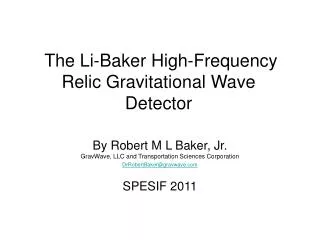
The Li-Baker High-Frequency Relic Gravitational Wave Detector. By Robert M L Baker, Jr. August 12, 2010, Sternberg Astronomical Institute of Moscow State University. Based In Part on the following Manuscript.

E N D
The Li-Baker High-Frequency Relic Gravitational Wave Detector By Robert M L Baker, Jr. August 12, 2010, Sternberg Astronomical Institute of Moscow State University
Based In Part on the following Manuscript “A new theoretical technique for the measurement of high-frequency relic gravitational waves” by R. Clive Woods, Robert M L Baker, Jr., Fangyu Li, Gary V. Stephenson, Eric W. Davis and Andrew W. Beckwith (Each has a specialized contribution with Baker primarily involved in the engineering design, e.g., Li-Baker detection chamber shape, absorbent walls, component arrangement, Herschelian telescope optics, system engineering, etc.)
INTRODUCTION • The measurement of High-Frequency Relic Gravitational Waves or HFRGWs could provide important information on the origin and development of our Universe. • There have been three instruments built to detect and measure HFRGWs, but so far none of them has the required detection sensitivity. • This lecture describes another detector, based on a new measurement technique, as referenced in the theoretical-physics literature, called Li-Baker detector . • Sensitivity as well as operational concerns, especially background noise, are discussed. • The potential for useful HFRGW measurement is theoretically confirmed.
What the Li-Baker Detector is Expected to Measure • The maximal signal and peak of HFRGWs expected from the beginning of our Universe, the “Big Bang,” by the quintessential inflationary models (Brustein, Gasperini, Giovannini and Veneziano 1995, Buonanno, Maggiore and Ungarelli 1997, de Vega, Mittelbrünn and Sanchez 1999, Giovannini 1999, Grishchuk 1999 and Beckwith 2009) and some string cosmology scenarios (Infante and Sanchez 1999, Mosquera and Gonzalez 2001, Bisnovatyi-Kogan and Rudenko 2004), may be localized in the gigahertz band near 10 GHz. • Their dimensionless spacetime strain intensities (m/m), h, vary from up to ~ 10-30 to ~ 10-34 Low-frequency gravitational wave detectors such as LIGO, which are based on interferometers, cannot detect HFRGWs (Shawhan 2004). • A frequency scancould reveal other HFRGW effects of interest in the early universe at a variety of HFRGW base frequencies other than 10 GHz.
Predicted relic gravitational wave energy density Ωgwas a function of frequency (slide 6, Grishchuk 2007) and Hubble parameter n
HFRGW Detectors Already Built • Three such detectors have been built (Garcia-Cuadrado 2009), utilizing different measurement techniques. And others proposed, for example by the Russians They are promising for future detection of HFRGWs having frequencies above 100 kHz (the definition of high-frequency gravitational waves or HFGWs by Douglass and Braginsky 1979), but their sensitivities are many orders of magnitude less than that required to detect and measure the HFRGWs so far theorized. • The following slides show the • The BirminghamHFGW detector that measures changes in the polarization state of a microwave beam (indicating the presence of a GW) moving in a waveguide about one meter across. It is expected to be sensitive to HFRGWs having spacetime strains of h ~2 × 10-13.
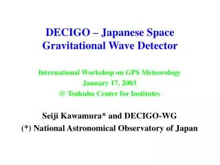
Additional Existing HFRGW Detectors • The second of these alternate detectors was built by the INFN Genoa, Italy. It is a resonant HFRGW detector, comprising two coupled, superconducting, spherical, harmonic oscillators a few centimeters in diameter. The oscillators are designed to have (when uncoupled) almost equal resonant frequencies. In theory, the system is expected to have a sensitivity to HFRGWs with intensities of about h ~ 2×10-17 with an expectation to reach a sensitivity of ~ 2 × 10-20. Details concerning the present characteristics and future potential of this detector, especially its frequency bands, can be found in Bernard, Gemme and Parodi 2001, Chincarini and Gemme 2003, and Ballantini et al. 2005. As of this date, however, there is no further development of the INFN Genoa HFRGW detector. • The third alternate detector is the Kawamura100 MHz HFRGW detector, which has been built by the Astronomical Observatory of Japan. It comprises two synchronous interferometers exhibiting arms lengths of 75 cm. Its sensitivity is h ≈ 10-16and its other characteristics can be found in Nishizawa et al. 2008.
Other HFRGW Detection Techniques • Another HFRGW detector, under development by the Russians (Mensky 1975; Mensky and Rudenko 2009), involves the detection of gravitational waves by their action on an electromagnetic wave in a closed waveguide or resonator. • Krauss, Scott and Meyer (2010) suggest that: “… primordial (relic) gravitational waves also leave indirect signatures that might show up in CMB (Cosmic Microwave Background) maps.” They suggest the use of thousands of new detectors (as many as 50,000) to obtain the required sensitivity.
Publications Presenting the Li-Effect or Li-Theory • Fangyu Li ‘s new theory, upon which the Li-Baker Detector is based, was first published in 1992 and subsequently aspects of it were published in the following prominent, well-respected and often cited, peer-review journals: • Physical Review D • InternationalJournal of Modern Physics B • The European Physical Journal C • InternationalJournal of Modern Physics D • Examples of the peer-reviewed journal articles include: • Fang-Yu Li, Meng-Xi Tang, Jun Luo, and Yi-Chuan Li (2000) “Electrodynamical response of a high energy photon flux to a gravitational wave,” Physical Review D, Volume 62, July 21, pp. 044018-1 to 044018 -9. • Fang-Yu Li, and Meng-Xi Tang, (2002), “Electromagnetic Detection of High-Frequency Gravitational Waves” International Journal of Modern Physics D 11(7), 1049-1059
Li-effect References • Fang-Yu Li, Meng-Xi Tang, and Dong-Ping Shi, (2003), “Electromagnetic response of a Gaussian beam to high-frequency relic gravitational waves in quintessential inflationary models,” Physical Review D 67, pp. 104006-1 to -17. • Fangyu Li and Robert M. L. Baker, Jr. (2007), “Detection of High-Frequency Gravitational Waves by Superconductors,” 6th International Conference on New Theories, Discoveries and Applications of Superconductors and Related Materials, Sydney, Australia, January 10; International Journal of Modern Physics B 21, Nos. 18-19, pp. 3274-3278. • Fangyu Li, Robert M L Baker, Jr., Zhenyun Fang, Gary V. Stephensonand Zhenya Chen (2008) (Li-Baker Chinese HFGW Detector), “Perturbative Photon Fluxes Generated by High-Frequency Gravitational Waves and Their Physical Effects,” The European Physical Journal C. 56, pp. 407-423. Paper with referee comments: http://www.drrobertbaker.com/docs/Li-Baker%206-22-08.pdf • Fangyu Li, N. Yang, Z. Fang, R. M L Baker, Jr., G. V. Stephenson and H. Wen, (2009), “Signal photon flux and background noise in a coupling electromagnetic detecting system for high-frequency gravitational waves,” Phys. Rev. D. 80, 060413-1-14 available at: http://www.gravwave.com/docs/Li,%20et%20al.%20July%202009,%20HFGW%20Detector%20Phys.%20Rev.%20D.pdf
Details of the Li Effect The Li Effect is very different from the well-known classical (inverse)Gertsenshtein (1962) effect. With the Li effect, a gravitational wave transfers energy to a separately generated electromagnetic (EM) wave in the presence of a static magnetic field. That EM wave, formed as a Gaussian beam (GB), has the same frequency as the GW and moves in the same direction. This is the “synchro-resonance condition,” in which the EM and GW waves are synchronized. It is unlike the Gertsenshtein effect, where there is no input EM wave that must be synchronized to the incoming gravitational wave. The result of the intersection of the parallel and superimposed EM and GW beams, according to the Li effect, is new EM photons moving off in a direction (both ways on the x-axis) perpendicular to the directions of the beams (GB and HFRGWs) on the z-axis and of the magnetic field (on the y-axis), as exhibited in a following slide. These photons signal the presence of HFGWs and are termed a “perturbative photon flux,” or PPF.
Li-effect detection photons directed to locations at both ends of the x-axis that are less affected by noise The result of the intersection of the parallel and superimposed EM and GW beams, according to the Li effect, is new EM photons moving off in a direction (both ways on the x-axis) perpendicular to the directions of the beams (GB and HFRGWs) on the z-axis and of the magnetic field (on the y-axis)
Gertsenshtein Effect It should be recognized thatunlike the Gertsenshtein effect, the Li effect produces a first-order perturbative photon flux (PPF) that is proportional to the amplitude of the gravitational wave (GW) intensity A (not A2). In the case of the Gertsenshtein effect, such photons are a second-order effect and according to equation (7) in Li, et al. (2009), the number of EM photons is “…proportional to the amplitude squared of the relic HFGWs, A2,” … and that it would be necessary to accumulate such EM photons for at least 1.4 × 10¹⁶ seconds in order to achieve relic HFGW detection utilizing the Gertsenshtein effect (Li et al. 2009). In the case of the Li effect the number of EM photons is proportional to the amplitude of the relic HFGWs, A ≈ 10-30, not its square, so that it would be necessary to accumulate such EM photons for only about 102 to 105 seconds in the transverse background photon noise fluctuation in order to achieve relic HFGW detection (Li, et al. 2009). The JASON report (Eardley 2008) confuses the two effects and erroneously suggests that the Li-Baker HFGW detector utilizes the inverse Gertsenshtein effect. The Li-Baker HFGW detector doesnot utilize the inverse Gertsenshtein effect, and it has a theoretical sensitivity that is about A/A2 = 1030 greater than the value incorrectly reported in the JASON report.
Theory of Operation • 1. A Gaussian microwave beam or GB (focused, with minimal side lobes and off-the-shelf microwave absorbers for effectively eliminating diffracted waves at the transmitter horn’s edges (“out of sight” of the microwave receivers) shown in yellow and blue in the slides) is aimed along the +z-axis at the same frequency as the intended HFGW signal to be detected . • 2. A static magnetic field B (generated typically using superconductor magnets such as those found in a conventional MRI medical body scanner) and installed linearly along the z-axis, is directed (N to S) along the y-axis • 3. Semi-paraboloid reflectors are situated back-to-back in the y-z plane to reflect the +x and –x moving PPF detection photons (on both sides of the y-z plane in the interaction volume) to the microwave receivers.
Theory of Operation Continued • 4. High-sensitivity, shielded microwave receivers are located at each end of the x-axis and below the GB entrance aperture to the Interaction Volume. Possible microwave receivers include an off-the-shelf microwave horn plus HEMT (High Electron Mobility Transistor) receiver; Rydberg Atom Cavity Detector (Yamamoto, et al. 2001) and single-photon detectors (Buller and Collins 2010). Of these, the HEMT receiver is recommended because of its off-the-shelf availability. • 5. A high-vacuum system able to evacuate the chamber from 10-6 to 10–11 Torr (nominally about 7.5 × 10⁻⁷ Torr) is utilized. This is well within the state of the art, utilizing multi-stage pumping, and is a convenient choice. Utilized to essentially eliminate GB scattering. • 6. A cooling system is selected so that the temperature T satisfies kBT << ћ, where kB is Boltzmann’s constant and T << ћ/kB 3K for detection at 10 GHz. This condition is satisfied by the target temperature for the detector enclosure T < 480mK, which can be conveniently obtained using a common helium-dilution refrigerator so very few thermal photons will be radiated at 10 GHz in the narrow bandwidth.
Equipment Layout Representative of an HFGW Detection System, Notional Picture of Stainless Steel and Titanium Vacuum/Cryogenic Containment Vessel and Faraday Cage for HFGW Detection on left; Shanghai Institute of Optics and Fine Mechanics (SIOM) set up for laser research; but similar to what the Li-Baker apparatus would look like.
Sensitivity The intersection of the magnetic field and the GB defines the “interaction volume” where the detection photons or PPF are produced. The interaction volume for the present design is roughly cylindrical in shape, about 30 cm in length and 9 cm across. In order to compute the sensitivity, that is the number of detection photons (PPF) produced per second for a given amplitude HFGW, we will utilize equation (7) of the analyses in Baker, Woods and Li (2006), which is a simplification of equation (59) in Li, et al. (2008), nx(1)= (1/μ0ћ ωe) AByψ0δs s-1(1) where nx(1) is the number of x-directed detection photons per second produced in the interaction volume (defined by the intersection of the Gaussian beam and the magnetic field) , ћ = Planck’s reduced constant, e = angular frequency of the EM (= 2πνe), νe = frequency of the EM, A = the amplitude of the HFGW (dimensionless strain of spacetime variation with time), By = y-component of the magnetic field, ψ0 = electrical field of the EM Gaussian beam or GB and δs is the cross-sectional area of the EM Gaussian beam and magnetic field interaction volume. For a proof-of-concept experiment, the neck of the GB is 20 cm out along the z-axis from the transmitter; the radius of the GB at its waist, W, is (λez/π)1/2 = (3 × 20/π)1/2 = 4.3 cm.
Sensitivity Continued The GB diameter is 8.6 cm (approximately the width of the interaction volume);and the length of the interaction volume is l = 30 cm, so δs = 2Wl = 2.58 × 10⁻² m2, i. e., the areas of the GB and By overlap. From the analysis presented in Li, Baker and Fang (2007), the electrical field of the EM GB, ψ, is proportional to the square root of EM GB transmitter power, which in the case of a 103 Watt transmitter is 1.26 × 10⁴ Vm-1. For the present case, νe = 1010 s-1, ωe = 6.28 × 10¹⁰ rad/s, A = 10-30, and By= 16 T. Thus equation (1) gives Nx(1) = 99.2 PPF detection photons per second. For a 103 second observation accumulation time interval or exposure time, there would be 9.92×10⁵ detection photons created, with about one-fourth of them focused at each receiver, since half would be directed in +x and half directed in the –x-directions respectively, and only about half of these would be focused on the detectors by paraboloid reflectors (the other half going the other way i.e., directed away from the focusing paraboloid reflectors and not sensed by the microwave receivers).
Standard quantum limit (SQL) - a result of the Heisenberg uncertainty principle There is another possible concern here: Stephenson (2009) concluded that a HFRGW intensity of hdet = 1.810–37m/m (strain in the fabric of space-time whose amplitude is A) represents the lowest possible GW strain variation detectable by each RF receiver in the Li-Baker HFGW detector. This limit is called “quantum back-action” or standard quantum limit (SQL) and is a result of the Heisenberg uncertainty principle. This sensitivity limit might be mitigated, however, by a “quantum-enhanced measurements using machine learning …” technique as discussed by Hentschel and Sanders (2010) and more specifically applied to optical interferometry as discussed by Steinberg (2010). An additional (1/2) factor increase in maximum sensitivity applies if the separate outputs from the two RF receivers are averaged, rather than used independently for false alarm reduction, resulting in a minimum hdet = 1.210–37 . Because the predicted best sensitivity of the Li-Baker detector in its currently proposed configuration is A = 10–30m/m, these results confirm that the Li-Baker detector is photon-signal-limited, not quantum-noise-limited; that is, the SQL is so low that a properly designed Li-Baker detector can have sufficient sensitivity to observe HFRGW of amplitude A 10–30 m/m.
Final Calculation (from Stephenson (2009) ) This is mostly due to the effective quality factor, Qr contribution arising from the synchro-resonance solution to the Einstein field equations that limit the PPF signal to a radiation pattern in certain directions, whereas noise is distributed uniformly. By utilizing directional antennas, the Li-Baker detector can capitalize upon this gain due to the focusing power of the semi-paraboloid mirror as a contribution to Q in angular space as well. This is calculated in detail, octant by octant, by Li et al. (2008). Page 24 of Li et al. summarizes this in terms of angular concentration onto the detector. A non-directional antenna corresponds roughly to solid angle 2steradians (one hemisphere), so that the effective antenna gain is estimated as (Q solid angle) = 2 sr/10-4sr = 6.3104. Therefore, the predicted maximum quality factor will be Qtotal = QrQ solid angle Qt = 2.11039 where Qr is the radialquality factor(as already noted the possibility of using the “labeling” of B and use of a resonance cavity in the interaction volume would also increase Q). This finally gives the Standard Quantum Limit (SQL) for stochastic GW detection at 10 GHz: hdet = (1/Q)1/2(ћ/E)1/2 = 1.810–37m/m. Please see Stephenson (2009) for detailed numerical calculations.
Noise The noise in the Li-Baker HFRGW detector is somewhat similar to that in any microwave receiver. The difference is that the HFRGW signal manifests itself in detection photons (PPF) created by the interaction of a very strong microwave beam and the GWs—the synchro-resonant GB. The presence of the microwave beam having the same frequency as the detection photons gives rise to noise that is generated by the beam and is termed background photon flux (BPF) or dark-background shot noise. This noise source is in addition to the usual microwave receiver noise. These noise sources have different origins within the Li-Baker detector. For example, Johnson noise has an origin in amplifiers and thermal noise has an origin in relatively warm components of the detector. In order to account for these diverse noise sources, we translated them through the detector to the actual microwave receiver's) and treat them there as “noise power,” W. Engineers term this noise equivalent power or NEP (Boyd 1983).
Gaussian Beam (GB) Noise A major source of noise in the Li-Baker detector is expected to be due to the GB. In the prototype Li-Baker HFRGW detector under analysis, which has peak sensitivity at 10 GHz, the energy per detection photon is hνe= 6.626 × 10⁻²⁴ J, while the HFRGWs or the Gaussian beam both have the same frequency for synchro-resonance. So for a 103 W GB, the total photons per second for the entire beam is 1.51 × 1026. A very large flux. The noise BPF from the scattering in the GB, hydrogen or helium is introduced into the detector enclosure prior to evacuating it to reduce the molecular cross-section and therefore increase the photon mean free path. scattering, λe =3 cm = 3 × 10⁸ Å (wavelength of the GB’s EM radiation) is much greater than the diameter of the He molecule (1 × 10⁻⁸ cm), so there would be Rayleigh scattering (caused by particles much smaller than the wave length of the EM radiation).
Scattering in the GB interaction volume We utilize the scattered intensity from a molecule with incident intensity Io as given by (Nave 2009) I = Io (8π4 α2/λ4R2)(1 + cos2θ) where is the atomic polarizability expressed as a polarization volume (where the induced electric dipole moment of the molecule is given by 4oE), is the scattering angle, and R is the distance from particle to detector. Note that the scattering is not isotropic (there is a -dependence) but in the present case, = 90° so the ratio of incident to scattered photon intensity is given by . The polarizability is 1.1 × 10⁻³⁰ m3 from Robb (1974) so the scattering intensity ratio is 1.2 × 10-49 for each atom in the chamber. The volume of interaction is about 2000 cm3 (30 cm long and roughly 8 cm 8 cm in area) so at a pressure reduced to its base value of 7.5 10–7 Torr at temperature 480 mK, the number of molecules contained is about 3 1016, giving a total scattering intensity ratio of 3.49 10–33. There are 1.51 1026 photons produced per second in the 103 W, 10 GHz GB. Therefore, in 103 s of observation time, the number of photons received from Rayleigh scattering in the interaction volume over one-thousand seconds is much less than 1, and again scattering will be negligible.
Microwave Absorbers Absorbers are of two types: metamaterial or MM absorbers, which have no reflection, only transmission (Landy, et al., 2008) and the usual commercially available absorbers in which there is reflection, but no transmission. In theory, multiple layers of metamaterials could result in a near “perfect” absorber (two layers absorb noise to 45dB over their specific frequency range 5 to10 GHz, according to Landy, et al. 2008 p. 3). But in practice, that might not be possible, so a combination of MMs (sketched as blue linesin the next two schematics of the detector) backed up by commercially available microwave absorbers, as shown in a subsequent slide (Patent Pending), is desirable. As Landy, et al. (2008) state. “In this study, we are interested in achieving (absorption) in a single unit cell in the propagation direction. Thus, our MM structure was optimized to maximize the [absorbance] with the restriction of minimizing the thickness. If this constraint is relaxed, impedance matching is possible, and with multiple layers, a perfect [absorbance] can be achieved.” In their study, the frequency range of 5 to 10 GHz is the same as that of the BPF from the GB.
Side-view schematic of the Li-Baker HFGW detector, exhibiting microwave-absorbent walls comprising an anechoic chamber
Reflectors Semi-paraboloid reflectors are situated back-to-back in the y-z plane, as shown in the slides, to reflect the +x and –x moving PPF detection photons (on both sides of the y-z plane in the interaction volume) to the microwave receivers. The sagitta or depth of such a reflector (60 cm effective aperture) is about 2.26 cm. Since this is greater than a tenth of a wavelength of the detection photons, λe/10 = 0.3 cm, such a paraboloid reflector is required, rather than a plane mirror (also, for enhanced noise elimination, the reflector’s focus is below the x axis and “out of sight” of the GB’s entrance opening). Thus the paraboloid mirrors are slightly tilted, which allows the focus to be slightly off-axis (similar to a Herschelian telescope) so that the microwave receivers cannot “see” the orifice of the Gaussian beam (GB) and, therefore, encounter less GB spillover noise. The reflectors can be constructed of almost any material that is non-magnetic (to avoid being affected by the intense magnetic field), reflects microwaves well and will not outgas in a high vacuum. The material of the reflectors can be in the form of fractal membranes that reflect more than 99 % of the incident microwaves
Plan-view schematic of the Li-Baker HFGW detector, exhibiting microwave-absorbent walls in the anechoic chamber.
Schematic of the multilayer metamaterial or MM absorbers and pyramid absorber/reflector. Patent Pending 1 Incident 2 1st metamaterial (MM) layer 3 transmitted 4 typical MM layer 6 conventional microwave absorber 8 reflected 10 remaining The incident ray can have almost any inclination: Service (2010)
Incidence Angle The absorption is by means of off-the-shelf -40 dB microwave pyramid reflectors/absorbers and by layers of metamaterial (MM) absorbers (tuned to the frequency of the detection photons -45 dB each double layer) shown in the slide (Patent Pending). The incident ray can have almost any inclination. As Service (2010) writes, “… Sandia Laboratories in Albuquerque, New Mexico are developing a technique to produce metamaterials that work with [electromagnetic radiation] coming from virtually any direction.” In addition, isolation from background noise is further improved by cooling the microwave receiver apparatus to reduce thermal noise background to a negligible amount. In order to achieve a larger field of view (the detector would be very sensitive to the physical orientation of the instrument) and account for any curvature in the magnetic field, an array of microwave receivers having, for example, 6 cm by 6 cm horns (two microwave wavelengths, or 2λe on a side) could be installed at x = ± 100 cm (arrayed in planes parallel to the y-z plane).
Engineering Calculation Optimized to Maximize the Absorbance We design an absorption “mat” (Patent Pending) for maximum absorbance consisting of two double MM layers, each layer a quarter wavelength from the next (to cancel any possible surface reflection), providing 45 dB 45 dB = 90 dB absorption. Behind these MM layers is a sheet of 10 GHz microwave pyramid absorbers, providing 40 dB absorption before reflection back into the three MM layers. Thus the total absorption is 90 dB 40 dB –90 dB = 220 dB or a reduction of 10-22 in the incident radiation.
Field of View In order to achieve a larger field of view (the detector would be very sensitive to the physical orientation of the instrument) and account for any curvature in the magnetic field, an array of microwave receivers having, for example, four 3 cm by 3 cm horns (i.e., a receiver array two microwave wavelengths, or 2λe on a side) could be installed at x = ± 100 cm (arrayed in planes parallel to the y-z plane).
Noise Equivalent Power (NEP) A standard sensor engineering-design method, already mentioned, for aggregating noise sources is to translate all noise terms through the system, or “refer them” from the location at which they occur to the equivalent noise at the detection photon microwave receiver(s) (Boyd 1983). Such an expression of noise is equivalent to the amount of power that this amount of noise would represent at the detector, and is known as the noise-equivalent power or NEP. All the uncorrelated noise components can be root-sum-squared together, so that: NEP = √ [(Pnd)2+(Pns)2 + (Pnj)2 + (Pnpa)2 + (Pnqa)2] W , where the equivalent-power noise components are defined as follows:
NEP Components The dark-background shot noise isPnd= hν√(Nd)/Δt and Ndis the dark-background- photon count. Shot noise is proportional to the square root of the number of photons present and diffraction and is mitigated by using the absorption mat and wall geometry to focus the detection photon (PPF) on detectors (microwave receivers) on a different location than the BPF background photons. Stray BPF spillover and diffraction that still manages to get reflected onto the detectors will create the shot noise, but such noise can be filtered out by pulse-modulating the magnetic field. The signal shot noise isPns= hν√(Ns)/Δt where Nsis the signal-photon count, and Δt is the sample or accumulation time. There is of course no way to mitigate signal photon noise because the creation and propagation of HFRGW photons is a cosmological process and this is one of the important measurements to be made.
NEP Components Continued The phase or frequency noise(of the EM-GB) is due to the fluctuations in the GB. Steps will need to be taken to keep the GB source tuned precisely to the interaction volume resonance, thus reducing phase noise and maximizing the resonant magnification effect required from the interaction volume cavity. A cavity-lock loop or alternatively a phase-compensating feedback loop will be selected during post-fabrication trials to mitigate this noise source The Johnson noise(due to the thermal agitation of electrons when they are acting as charge carriers in a power amplifier) is Pnj = 4kBTRLBW, where RLis the equivalent resistance of the front-end amplifier and BW is the bandwidth. Mitigation of this noise source is accomplished by reducing bandwidth or reducing load resistance. However, in practice the bandwidth is often fixed by the application, in this case by the detection bandwidth. And the load resistance is required to generate a large voltage from a very small current. Hence there is in practice an optimum selection of load resistance that will optimize the signal to noise output, and the selection of this load resistance is the essence of impedance matching in its most basic form. Johnson noise is generally reduced or eliminated also by refrigeration.
NEP Components Continued • The preamplifier noise is Pnpa= BW/ f1, which is essentially 1/f noise, where the crossover frequency f is related to stray capacitance and load resistance; in which f1 = 1/(2π RLCjn), where Cjn = detection capacitance plus FET (field effect transistor) input capacitance plus stray capacitance. This noise source is mitigated by reducing bandwidth, reducing load resistance, or reducing stray capacitance. • The quantization noise is Pnqa = QSE/ √12, where QSE is the quantization step equivalent or the value of one LSB (Least Significant Bit , the smallest value that is quantized by an ADC, or Analog to Digital Converter). This noise source is easily eliminated by increasing the number of bits used in an ADC so that the LSB is a smaller portion of the overall signal. In practice the QSE is selected so that it does not cause lower SNR.
Other Noise Sources • The mechanical thermal noise is caused by the Brownian motion of sensor components. Mitigation or elimination is to refrigerate the sensing apparatus to reduce thermal inputs. The 0.48 K cooling should be sufficient, but if not an even lower temperature can be achieved. • The sum of all these noise sources or noise equivalent power at the receiver(s) or NEP, is not a constant, but exhibits a stochastic or random component. In order to obtain the best estimate of the detection photons one would need to utilize a filter, possibly a Kalman filter (pp. 376-387 in Baker 1967). Only the noise -- not the signal or detection photons (PPF) -- is present when the magnetic field is turned off, so the noise can be “labeled.”
Results • The total NEP from Eq. (4.4) of 1.02×10⁻²⁶is Quantization and thermal noise limited at roughly 1×10-26 to 2×10-27 W for a temperature of 0.48K. If need be the receivers could be further cooled and shielded from noise by baffles in which the spherical BPF wave front if significant, can be reduced by baffle diffraction and the PPF focused by the reflectors passed through the baffle openings with less interaction with baffle edges and less diffraction. Given a signal that exhibits the nominalvalue of 99.2 s-1 photons, one quarter of which is focused on each of the microwave receivers, which is 24.8 s-1 photons or 1.6×10⁻²² W, the signal-to-noise ratio for each receiver is better than 1500:1.
CONCLUSIONS • Three HFGW detectors have previously been fabricated, but analyses of their sensitivity and the results provided herein suggest that for meaningful relic gravitational wave (HFRGW) detection, greater sensitivity than those instruments currently provide is necessary. • The theoretical sensitivity of the Li-Baker HFGW detector studied herein, and based upon a different measurement technique than the other detectors, is predicted to be A = 10-30 m/m at a frequency of 10 GHz. • This detector design is not quantum-limited and theoretically exhibits sensitivity sufficient for useful relic gravitational wave detection. • Utilization of magnetic-field pulsed modulation allows for reduction in some types of noise. Other noise effects can only be estimated based on the Li-Baker prototype detector tests, and some of the design and adjustments can only be finalized during prototype fabrication and testing. • The detector can be built from off-the-shelf, readily available components and its research results would be complementary to the proposed low-frequency gravitational wave (LFGW) detectors, such as the Advanced LIGO, Russian Project OGRAN and the proposed Laser Interferometer Space Antenna or LISA.
Bandwidth • Bandwidth (BW) is determined by two factors: • The Gaussian Beam can be adjusted to have a peak frequency spread of from a few Hz to MHz so that HFRGWs of only this frequency range or band will produce PPF or detection microwave photons. Of course random fluctuations in the transmitter output cause BW broadening. • The microwave detectors can also be tuned to a similar frequency range or band. In general, the narrower the frequency range or bandwidth is the more sensitive is the detector (the noise floor is lowered at smaller BW). Frequency scanning allows for a wide band of HFRGWs to be analyzed however. As an example, if there was a 1 Hz “bandwidth” and a 1000s observation interval, then over a year of observation about a 30kHz HFRGW frequency band could be scanned or if 100s interval, then a 300 kHz band of HFRGWs could be scanned. If a 1 kHz BW, then a 10 ± 0.15 GHz band could be scanned using 100s intervals in a year. The detector can also have a different base frequency, such as less than one GHz or greater than one-hundred GHz, by changing the frequency of the GB and retuning (or replacing) the receivers and microwave absorbing walls and modifying the refrigeration to a different temperature.
Detector Parameter Selection • In the following Tables are to be found parameterized values of the detection photons per second or photon flux or signal. A different choice of parameters and more sensitive receivers than the off-the-shelf microwave horn plus HEMT receiver could increase the sensitivity by two or three orders of magnitude. Table 1 provides values for an interaction volume cross section of δs = 0.1 m x 0.05 m = 0.005 m2, Table 2 for δs = 0.30 m x 0.086 m = 0.0258 m2 (the nominal case) and Table 3 for δs = 6 m x 0.5 m = 1.5 m2 . Table 3 is valid under the assumption that the near–field approximation of Eq. (1) still holds and account is taken of the spreading property of the GB. If a dimension of the interaction volume is very long, for example over one meter, then the computation of the total transverse detection photon flux (signal) should be the result of an integration of Eq. (59) of Li et al. (2008), specifically, the numerical integration of the coefficients in Eqs. (60). A long interaction volume would also incur a higher cost due to a more complex and expensive magnet system.
Table 1. A table containing the detection photons per second s-1 for various values of Byand transmitter power for δs = 0.005 m2.
Table 2. A table containing the detection photons per second s-1 for various values of Byand transmitter power for δs = 0.0258 m2. The nominal case,
Table 3. A table containing the detection photons per second s-1 for various values of Byand transmitter power for δs = 1.5 m2.
Fangyu Li’s explanation of the peak region of the high-frequency relic GWs (HFRGWs) in the GHz band “Except for the quintessential inflationary models (QIM), the pre-big bang model (PBB) and the ekpyrotic scenario all models expected that the maximal signal and peak of the HFRGWs may be localized in the GHz band. The difference is that the peak bandwidth of the PBB is much larger than that of the QIM. The former is from 10Hz to 10GHz (B.P. Abbott et al, Nature 460 (2009) 990), the latter is from 1GHz to 10GHz (M. Giovannini, Phys. Rev. D60 (1999) 123511).”