Download
1 / 41
410 likes | 741 Views
One-Minute Survey Result. Thank you for your responses Kristen, Anusha, Ian, Christofer, Bernard, Greg, Michael, Shalini, Brian and Justin Valentine’s challenge Min: 30-45 minutes, Max: 5 hours, Ave: 2-3 hours Muddiest points Regular tree grammar (CS410 compiler or CS422: Automata)

E N D
One-Minute Survey Result Thank you for your responses Kristen, Anusha, Ian, Christofer, Bernard, Greg, Michael, Shalini, Brian and Justin Valentine’s challenge Min: 30-45 minutes, Max: 5 hours, Ave: 2-3 hours Muddiest points Regular tree grammar (CS410 compiler or CS422: Automata) Fractal geometry (“The fractal geometry of nature” by Mandelbrot) Seeing the Connection Remember the first story in Steve Jobs’ speech “Staying Hungry, Staying Foolish”? In addition to Jobs and Shannon, I have two more examples: Charles Darwin and Bruce Lee EE465: Introduction to Digital Image Processing
Data Compression Basics Discrete source Information=uncertainty Quantification of uncertainty Source entropy Variable length codes Motivation Prefix condition Huffman coding algorithm EE465: Introduction to Digital Image Processing
Information • What do we mean by information? • “A numerical measure of the uncertainty of an experimental outcome” – Webster Dictionary • How to quantitatively measure and represent information? • Shannon proposes a statistical-mechanics inspired approach • Let us first look at how we assess the amount of information in our daily lives using common sense EE465: Introduction to Digital Image Processing
Information = Uncertainty Zero information Pittsburgh Steelers won the Superbowl XL (past news, no uncertainty) Yao Ming plays for Houston Rocket (celebrity fact, no uncertainty) Little information It will be very cold in Chicago tomorrow (not much uncertainty since this is winter time) It is going to rain in Seattle next week (not much uncertainty since it rains nine months a year in NW) Large information An earthquake is going to hit CA in July 2006 (are you sure? an unlikely event) Someone has shown P=NP (Wow! Really? Who did it?) EE465: Introduction to Digital Image Processing
Shannon’s Picture on Communication (1948) channel encoder channel decoder source channel destination super-channel source encoder source decoder The goal of communication is to move information from here to there and from now to then Examples of source: Human speeches, photos, text messages, computer programs … Examples of channel: storage media, telephone lines, wireless transmission … EE465: Introduction to Digital Image Processing
Source-Channel Separation Principle* The role of channel coding: Fight against channel errors for reliable transmission of information (design of channel encoder/decoder is considered in EE461) We simply assume the super-channel achieves error-free transmission The role of source coding (data compression): Facilitate storage and transmission by eliminating source redundancy Our goal is to maximally remove the source redundancy by intelligent designing source encoder/decoder EE465: Introduction to Digital Image Processing
Discrete Source A discrete source is characterized by a discrete random variable X Examples Coin flipping: P(X=H)=P(X=T)=1/2 Dice tossing: P(X=k)=1/6, k=1-6 Playing-card drawing: P(X=S)=P(X=H)=P(X=D)=P(X=C)=1/4 What is the redundancy with a discrete source? EE465: Introduction to Digital Image Processing
Two Extreme Cases source encoder source decoder tossing a fair coin channel P(X=H)=P(X=T)=1/2: (maximum uncertainty) Minimum (zero) redundancy, compression impossible HHHH… Head or Tail? tossing a coin with two identical sides channel duplication TTTT… P(X=H)=1,P(X=T)=0: (minimum redundancy) Maximum redundancy, compression trivial (1bit is enough) Redundancy is the opposite of uncertainty EE465: Introduction to Digital Image Processing
Quantifying Uncertainty of an Event Self-information • probability of the event x • (e.g., x can be X=H or X=T) notes must happen (no uncertainty) 0 1 unlikely to happen (infinite amount of uncertainty) 0 Intuitively, I(p) measures the amount of uncertainty with event x EE465: Introduction to Digital Image Processing
Weighted Self-information 0 0 1/2 1 1/2 0 1 0 As p evolves from 0 to 1, weighted self-information first increases and then decreases Question: Which value of p maximizes Iw(p)? EE465: Introduction to Digital Image Processing
Maximum of Weighted Self-information* p=1/e EE465: Introduction to Digital Image Processing
Quantification of Uncertainty of a Discrete Source • A discrete source (random variable) is a collection (set) of individual events whose probabilities sum to 1 X is a discrete random variable • To quantify the uncertainty of a discrete source, we simply take the summation of weighted self-information over the whole set EE465: Introduction to Digital Image Processing
Shannon’s Source Entropy Formula (bits/sample) or bps Weighting coefficients EE465: Introduction to Digital Image Processing
Source Entropy Examples • Example 1: (binary Bernoulli source) Flipping a coin with probability of head being p (0<p<1) Check the two extreme cases: As p goes to zero, H(X) goes to 0 bps compression gains the most As p goes to a half, H(X) goes to 1 bps no compression can help EE465: Introduction to Digital Image Processing
Entropy of Binary Bernoulli Source EE465: Introduction to Digital Image Processing
Source Entropy Examples N • Example 2: (4-way random walk) W E S EE465: Introduction to Digital Image Processing
Source Entropy Examples (Con’t) • Example 3: (source with geometric distribution) A jar contains the same number of balls with two different colors: blue and red. Each time a ball is randomly picked out from the jar and then put back. Consider the event that at the k-th picking, it is the first time to see a red ball – what is the probability of such event? Prob(event)=Prob(blue in the first k-1 picks)Prob(red in the k-th pick ) =(1/2)k-1(1/2)=(1/2)k EE465: Introduction to Digital Image Processing
Source Entropy Calculation If we consider all possible events, the sum of their probabilities will be one. Check: Then we can define a discrete random variable X with Entropy: Problem 1 in HW3 is slightly more complex than this example EE465: Introduction to Digital Image Processing
Properties of Source Entropy • Nonnegative and concave • Achieves the maximum when the source observes uniform distribution (i.e., P(x=k)=1/N, k=1-N) • Goes to zero (minimum) as the source becomes more and more skewed (i.e., P(x=k)1, P(xk) 0) EE465: Introduction to Digital Image Processing
History of Entropy • Origin: Greek root for “transformation content” • First created by Rudolf Clausius to study thermodynamical systems in 1862 • Developed by Ludwig Eduard Boltzmann in 1870s-1880s (the first serious attempt to understand nature in a statistical language) • Borrowed by Shannon in his landmark work “A Mathematical Theory of Communication” in 1948 EE465: Introduction to Digital Image Processing
A Little Bit of Mathematics* • Entropy S is proportional to log P (P is the relative probability of a state) • Consider an ideal gas of Nidentical particles, of which Ni are in the i-th microscopic condition (range) of position and momentum. • Use Stirling’s formula: log N! ~ NlogN-N and note that pi = Ni /N, you will get S ~ ∑ pi log pi EE465: Introduction to Digital Image Processing
Entropy-related Quotes “My greatest concern was what to call it. I thought of calling it ‘information’, but the word was overly used, so I decided to call it ‘uncertainty’. When I discussed it with John von Neumann, he had a better idea. Von Neumann told me, ‘You should call it entropy, for two reasons. In the first place your uncertainty function has been used in statistical mechanics under that name, so it already has a name. In the second place, and more important, nobody knows what entropy really is, so in a debate you will always have the advantage. ” --Conversation between Claude Shannon and John von Neumann regarding what name to give to the “measure of uncertainty” or attenuation in phone-line signals (1949) EE465: Introduction to Digital Image Processing
Other Use of Entropy • In biology • “the order produced within cells as they grow and divide is more than compensated for by the disorder they create in their surroundings in the course of growth and division.” – A. Lehninger • Ecological entropy is a measure of biodiversity in the study of biological ecology. • In cosmology • “black holes have the maximum possible entropy of any object of equal size” – Stephen Hawking EE465: Introduction to Digital Image Processing
What is the use of H(X)? Shannon’s first theorem (noiseless coding theorem) For a memoryless discrete source X, its entropy H(X) defines the minimum average code length required to noiselessly code the source. Notes: 1. Memoryless means that the events are independently generated (e.g., the outcomes of flipping a coin N times are independent events) 2. Source redundancy can be then understood as the difference between raw data rate and source entropy EE465: Introduction to Digital Image Processing
Code Redundancy* Theoretical bound Practical performance li: the length of codeword assigned to the i-th symbol Average code length: Note: if we represent each symbol by q bits (fixed length codes), Then redundancy is simply q-H(X) bps EE465: Introduction to Digital Image Processing
How to achieve source entropy? entropy coding binary bit stream discrete source X P(X) Note: The above entropy coding problem is based on simplified assumptions are that discrete source X is memoryless and P(X) is completely known. Those assumptions often do not hold for real-world data such as images and we will recheck them later. EE465: Introduction to Digital Image Processing
Data Compression Basics • Discrete source • Information=uncertainty • Quantification of uncertainty • Source entropy • Variable length codes • Motivation • Prefix condition • Huffman coding algorithm EE465: Introduction to Digital Image Processing
Variable Length Codes (VLC) Recall: Self-information It follows from the above formula that a small-probability event contains much information and therefore worth many bits to represent it. Conversely, if some event frequently occurs, it is probably a good idea to use as few bits as possible to represent it. Such observation leads to the idea of varying the code lengths based on the events’ probabilities. Assign a long codeword to an event with small probability Assign a short codeword to an event with large probability EE465: Introduction to Digital Image Processing
4-way Random Walk Example variable-length codeword fixed-length codeword pk symbol k 0.5 S 00 0 N 0.25 01 10 E 0.125 10 110 W 0.125 11 111 symbol stream : S S N W S E N N N W S S S N E S S 32bits fixed length: 00000111001001011100000001100000 variable length: 28bits 0010111011010101110001011000 4 bits savings achieved by VLC (redundancy eliminated) EE465: Introduction to Digital Image Processing
Toy Example (Con’t) • source entropy: =0.5×1+0.25×2+0.125×3+0.125×3 =1.75 bits/symbol • average code length: Total number of bits (bps) Total number of symbols fixed-length variable-length EE465: Introduction to Digital Image Processing
Problems with VLC • When codewords have fixed lengths, the boundary of codewords is always identifiable. • For codewords with variable lengths, their boundary could become ambiguous S S N W S E … symbol VLC e S 0 00111010… N 1 00111010… 00111010… 10 E d d 11 S S W N S E … S S N W S E … W EE465: Introduction to Digital Image Processing
Uniquely Decodable Codes • To avoid the ambiguity in decoding, we need to enforce certain conditions with VLC to make them uniquely decodable • Since ambiguity arises when some codeword becomes the prefix of the other, it is natural to consider prefix condition Example: p pr pre pref prefi prefix ab: a is the prefix of b EE465: Introduction to Digital Image Processing
Prefix condition No codeword is allowed to be the prefix of any other codeword. We will graphically illustrate this condition with the aid of binary codeword tree EE465: Introduction to Digital Image Processing
Binary Codeword Tree root # of codewords Level 1 1 0 2 Level 2 11 10 01 00 22 … … Level k 2k EE465: Introduction to Digital Image Processing
Prefix Condition Examples symbol x codeword 1 codeword 2 S 0 0 N 1 10 10 110 E W 11 111 1 0 1 0 11 10 01 00 11 10 111 110 … … … … codeword 1 codeword 2 EE465: Introduction to Digital Image Processing
How to satisfy prefix condition? • Basic rule: If a node is used as a codeword, then all its descendants cannot be used as codeword. 1 0 Example 11 10 111 110 … EE465: Introduction to Digital Image Processing
Property of Prefix Codes Kraft’s inequality li: length of the i-th codeword (proof skipped) Example symbol x VLC- 1 VLC-2 S 0 0 1 10 N 10 110 E W 11 111 EE465: Introduction to Digital Image Processing
Two Goals of VLC design • achieve optimal code length (i.e., minimal redundancy) For an event x with probability of p(x), the optimal code-length is , where x denotes the smallest integer larger than x (e.g., 3.4=4 ) –log2p(x) code redundancy: Unless probabilities of events are all power of 2, we often have r>0 • satisfy prefix condition EE465: Introduction to Digital Image Processing
Solution: Huffman Coding (Huffman’1952) – we will cover it later while studying JPEG Arithmetic Coding (1980s) – not covered by EE465 but EE565 (F2008) EE465: Introduction to Digital Image Processing
Golomb Codes for Geometric Distribution Optimal VLC for geometric source: P(X=k)=(1/2)k, k=1,2,… codeword 0 10 110 1110 11110 111110 1111110 11111110 … … k 1 2 3 4 5 6 7 8 … 0 1 1 0 1 0 1 0 … EE465: Introduction to Digital Image Processing
Summary of Data Compression Basics Shannon’s Source entropy formula (theory) Entropy (uncertainty) is quantified by weighted self-information VLC thumb rule (practice) Long codeword small-probability event Short codeword large-probability event bps EE465: Introduction to Digital Image Processing