Download
1 / 80
800 likes | 805 Views
Sec. 2: Factor Analysis Ewart A.C. Thomas Psych 253 e.g., http :// en.wikipedia.org /wiki/ Factor_analysis. Quote from a ‘ mixed-models ’ thread, 4/13/12.

E N D
Sec. 2: Factor Analysis Ewart A.C. Thomas Psych 253 e.g., http://en.wikipedia.org/wiki/Factor_analysis
Quote from a ‘mixed-models’ thread, 4/13/12 “There are ways of modelling multiple outcomes simultaneously (see the MCMCglmm documentation on Multi-response models at http://cran.md.tsukuba.ac.jp/web/packages/MCMCglmm/vignettes/CourseNotes.pdf), but nine is a lot. Perhaps an exploratory factor analysis[emphasis added] could help you reduce the nine items to a smaller and more manageable number?” …
From Desmond Ong’s Frisem of his 2013 FYP (4/12/13): A person plays a roulette wheel with 3 possible outcomes, R, B, Y, with probs pr, pb, py. Given the outcome of the play, how much of 9 emotions is the person likely to feel? Outcome Emotion, Where ‘outcome’ has at least 5 dimensions, and ‘emotion’ may have as many as 9!
A brief digression - from HW-2Reliability of 1- vsk-item tests • What motivates this distinction? • Consider a reliability analysis based on a p (patients) x k (raters) matrix of scores. After this analysis, the rating method is applied to ‘many’ patients. Is a patient to be rated by 1 clinician? OR, is a patient rated by k = 2 or 4 clinicians, whose ratings are ‘pooled’ to assess the patient’s status? • The former leads us to report the reliability of a 1-item test; the latter that of a k-item test.
X1 X2 X3 X4 X5 X6 Factor 1 Factor 2 • A factor in Factor Analysis is said to exist when the various indicators, Xj, of the supposedly latent construct cohere, i.e., ‘hang together’. This notion of coherence is another appeal to consistency.
Outline • Class demo of Exploratory Factor Analysis (EFA) using B. Malle’s data on how we represent the ‘self’ • Describe data and goals of analysis • Then, before demo, review terminology, issues • P’s rate themselves on 32 traits, e.g., ‘distant’, ‘relaxed’, … We know we won’t theorise about 32 dimensions of personality. But what are the (2-6?) underlying (i.e., latent) dimensions (or factors) of personality? • To discover them, use correls, SPSS or R (Science), and lots of interpretation (Art)
Goals of analysis • How manylatent factors account for “most of” the variation among the observed traits or variables? • Which traits define each factor; hence what labels should we give each factor? • If the observed covariation can be explained by a small number of factors (e.g., 2-5), this would increase our understanding of the relationships among the traits or variables. • SPSS commands: Analyze > Dimension Reduction > Factor; enter the variables to be analyzed; click on Extraction, Rotation, Scores or Options as needed.
The base package in R has a function, factanal(), for doing FA. This function uses ‘maximum likelihood’ (ML, as opposed to, say, ‘principal components’, PC) to derive the factors. • When ML is used, there exists a [conservative] significance test for the null hypothesis that the k extracted factors are sufficient. This is convenient. • The package, ‘psych’, has a function, fa(), for doing FA. And there are many other functions!
Terminology (in prep for demo) • Communality of a variable; Factor; factor loading of a variable; variance accounted for by a factor; factor score coefficients for factorj; factor score of Personi. • Eigenvalues (= Sum of Squared loadings) • Rule-of-thumb: Factor j is important if its eigenvalue is greater than 1 (the average) • Interpretation of factors; rotation of factors • Composite variables = informal ‘factors’ defined by researcher, not by a formal FA
Communality of a variable = % variance explained by the m extracted factors = variance ‘in common’ with other variables Communalities Initial Extraction distant 1.000 .571 talkatv 1.000 .689 carelss 1.000 .690 hardwrk 1.000 .638 anxious 1.000 .680 agreebl 1.000 .576 tense 1.000 .735
Defn. of a FACTOR • A latent construct that 'causes' the observed variables, to a greater or lesser extent. Algebraically, a factor is estimated by a linear combination of observed variables. • When the ‘best-fitting’ factors are found, these factors are not unique. Any rotation of the best-fitting factors is also best-fitting. • Criterion of ‘interpretability’: To be useful, factors should be interpretable. Among equally ‘good’ rotations, select the rotation that yields the ‘best’ interpretation of the factors.
Example of rotation • Consider a case where the loadings on 8 variables in the (X, Y) coordinate system are all moderate or larger. That is, each variable loads on both factors, X and Y. In this case it is difficult to interpret X and Y. • Suppose, however, we rotate the axes to new orthogonal axes, (X’, Y’), such that variables load high on one factor and low on the other. It is now easy to interpret X’ and Y’ … • This is shown in the next slide.
Class demo (cont’d) • Exploratory Factor Analysis (EFA) using B. Malle’s data on how we represent the ‘self’ • P’s rate themselves on 32 traits, e.g., ‘distant’, ‘relaxed’, … We know we won’t theorise about 32 dimensions of personality. But what are the (2-6?) underlying (i.e., latent) dimensions (or factors) of personality? • Switch to the R console
Lecture 2.2: Points of emphasis in FA demo • ?factanal(): method = ML; default is to rotate with ‘varimax’; choose number, m, of factors to extract • ‘uniqueness’, which lies in (0, 1) • Test of sufficiency of m factors • Loadings for 1st few factors; interpret, label factors • Compare rotated with unrotated solutions
Loadings in rotated solution: Interpret Factors 1 & 2 Factor1 Factor2 distant 0.586 talkatv -0.760 hardwrk0.700 anxious agreebl outgoin -0.834 shy 0.724 discipl 0.698 persevr0.598 friendl -0.504 lazy -0.664
Loadings in unrotated solution: Interpret Factors 1’ & 2’ Factor1’ Factor2’ distant 0.581 talkatv -0.500 hardwrk 0.461 anxious agreebl outgoin -0.688 shy 0.620 discipl 0.486 persevr friendl -0.613 lazy 0.530
X1 X2 X3 X4 X5 X6 Factor 1 Factor 2 • A factor in Factor Analysis is said to exist when the various indicators, Xj, of the supposedly latent construct cohere, i.e., ‘hang together’. This notion of coherence is another appeal to consistency. u3 u1 v3
Return to terminology:FACTOR LOADING of a variable • For a model with 2 factors, F1 and F2, the i’th observed variableis (previous Slide): Xi = uiF1 + viF2 + ei. • The path coefficients, ui and vi, are the loadings of Xi on factors, F1 and F2, respectively.
VARIANCE accounted for by a factor • The amount of common variance for a set of observed variables that is explained by the factor. • The 1st factor extracted in most methods explains more variance than the remaining factors.
FACTOR SCORE COEFFICIENTS, or FACTOR WEIGHTS • A factor is estimated by a linear combination of observed variables, F = ∑wiXi. The set of weights, {wi}, for each factor gives the factor score coefficients for that factor.
FACTOR SCORE OF A PERSON Let xijbe the score of person j on variable i. Then is the factor score for person j on factor F. It can be seen that a person's factor score is a specific linear combination of that person's observed scores on all variables.
Eigenvalues • The k'th eigenvalue is equal to the variance accounted for by the k'th most important factor. The eigenvalues are used to compute the % variance accounted for by a factor, and the cumulative % variance accounted for by the first l factors.
INTERPRETATION: ROTATION OF FACTORS • Interpret a factor by which variables have ‘high’ loadings (positive or negative) on the factor. • Unrotated factors, usually the PC’s, often are more difficult to interpret than rotated factors. Rotation is a technique for improving the interpretability of factors. • If m PC’s are extracted and these m PC’s are then rotated to define m rotated factors, the m rotated factors explain exactly the same amount of variance as do the m PC’s.
The definition and interpretation of PC’s are not affected by how many PC’s are extracted. Each PC is a specific linear combination of all the variables. • However, the interpretation of, say, the 1strotated factor might depend on how many factors are extracted, because rotation changes the loadings. • Redundant or synonymous variables hinder the extraction of general factors. Combine them into composites, if possible.
Composites of synonymous variables • SHY = sum or average of {distant, shy, quiet, withdrawn} • TALKATIVE = {talkative, outgoing} • ANXIOUS = {anxious, tense, worrying}. Etc. • Using such composites (along with the non-redundant original variables) in the Factor Analysis reduces the number of redundant variables. Fewer specific factors & more general factors, are extracted. The latter advance theorizing.
FACTOR ANALYSIS IN R • The function, factanal(), produces a factor analysis in R. Principal Components Analysis (PCA, a more theoretically grounded version of Factor Analysis) can be done with prcomp() and princomp(). The file, ‘sfactanal1.r’, yields an analysis of Malle’s data. • #Factor analysis of Malle's data • d = read.table("personality0.txt") • res1 = factanal(d, factors=10, na.action=na.omit) • print(res1$loadings)
The classification problem: An introduction to multinomial logistic regression with mlogit() • Each S gives 32 self-ratings; raters then classify each S into one of 3 categories, e.g., for job training (management/tech/other) • Each trial is characterised by the activity levels of 32 (or 3200) voxels; we wish to determine which object category (e.g., ‘face’, ‘house’) was presented on each trial. • Use FA to reduce dimensionality of IV’s from 32 to k (= 4 or 5?). DV is categorical.
Logistic Model • Possible responses, j, are A, B, C (j = 1, 2, 3). Choose 1 category, e.g., ‘1’ as baseline. • pij= Prob(i’th S is classified as a j). How to model pij? • For Si, the j’th category has a latent strength, Uij; set Ui1 = 0 (for baseline).
Thus, for j > 1, it follows that loge(pij/pi1) = Uij. This is the multinomial logistic model – the log odds of choosing category j over category 1 is linear in Uij. To flesh it out, we assume that Uij is influenced by S’s traits: Our goal is to estimate the parameters, {bij}.
HW-3, #4: intro to mlogit() • Consider binary classifications, for simplicity. So mlogit() results could be obtained in the usual way with glm(…, family=binomial,…). But mlogit() applies to multinomial and mixed models!
Sources CITY AND REGIONAL PLANNING 775 Discrete-Choice Logit Models with R Philip A. Viton April 15, 2012 1. Most general, including mixed mlogit models: http://facweb.knowlton.ohio-state.edu/pviton/courses2/crp775/775-mlogit.pdf 2. Models with only participant-specific (i.e., individual-specific) variables: http://www.ats.ucla.edu/stat/r/dae/mlogit.htm 3. After installing “mlogit” and loading it with library(mlogit), use help(), as in “R > ?mFormula”.
d = read.csv("person.option2.vars.csv") #separate self-ratings in d0 for FA d0 = d[, c(1:32)]; d1 = d[, c(33:37)] #Do FA res1 = factanal(d0, factors=4, rotation="varimax", na.action=na.omit, scores= 'r') #print(res1$loadings, cutoff=.4) #to interpret PC’s d1$PC1 = res1$scores[,1]; d1$PC2 = -res1$scores[,2] d1$PC3 = res1$scores[,3]; d1$PC4 = res1$scores[,4] #PC1 = extravert, PC2 = conscientious, #PC3 = agreeable, PC4 = neurotic print(head(d1))
print(head(d1)) rating2 attr1.A attr1.B attr2.A attr2.B PC1 PC2 PC3 PC4 1 0 0.95 -0.01 -1.08 0.24 -1.23 -0.69 2.38 0.99 2 1 -0.29 0.02 -0.95 0.30 0.46 -0.11 0.80 -0.11 3 0 1.33 -0.08 0.16 0.11 -0.64 -0.79 1.71 -1.44 4 0 0.95 0.25 -0.86 -0.13 -0.08 0.11 0.99 -0.42 5 0 1.25 -0.32 -0.13 -0.55 -2.34 -0.20 -1.91 0.55 6 0 0.30 0.31 -0.54 -0.05 -1.16 -0.84 0.74 1.23 d10 = mlogit.data(d1, choice = "rating2", varying = c(2:5), shape = "wide") #reshape data for mlogit() print(head(d10)) rating2 PC1 PC2 PC3 PC4 alt attr1 attr2 chid 1.A TRUE -1.23 -0.69 2.4 0.99 A 0.9499 -1.08 1 1.B FALSE -1.23 -0.69 2.4 0.99 B -0.0061 0.24 1 2.A FALSE 0.46 -0.11 0.8 -0.11 A -0.2923 -0.95 2 2.B TRUE 0.46 -0.11 0.8 -0.11 B 0.0157 0.30 2 3.A TRUE -0.64 -0.79 1.7 -1.44 A 1.3303 0.16 3 3.B FALSE -0.64 -0.79 1.7 -1.44 B -0.0758 0.11 3
res1 = mlogit(rating2 ~ 1 | PC1 + PC2 + PC3 + PC4, d10) print(summary(res1)) #Redo with familiar binary logistic regression using glm(..., family = binomial, ...), data = d1 #Results are the same res1a = glm(rating2 ~ PC1 + PC2 + PC3 + PC4, family = binomial, d1) print(summary(res1a)) End of lecture
Lecture 2.3. Introduction to mlogit() • Task 1: Classify Si’s, who vary in {PC1, …, PC4}, as ‘A’ or ‘B’ (Yi = 0 or 1). In addition, on each classification the options, ‘A’ and ‘B’, are assigned attributes, e.g., ‘value’ or ‘scarcity’. • How does Y depend on the person-specific attributes, PCj, and on the option-specific attributes, e.g., ‘value’? • Task 2: S’s choose between an object of category ‘A’ (Yi = 0) and one of category ‘B’ (Yi = 1). How does Y depend on the person-specific and option-specific attributes? • These tasks are formally the same.
In Decision Theory, the models are usually stated as models of choice, rather than classification. Each S must choose one object from a set of objects. E.g. the set might be (i) {local, out-of- state, overseas} vacation; (ii) {immediate vs delayed} reward; (iii) {air, train, car, other} mode. To simplify, suppose the choice set is {A vs B} object. Each object has attributes that vary within and between choice sets; e.g., price, cost, quality, risk, reward, etc. To simplify, suppose each object has 2 attributes, (attr1, attr2) or (X, Y).
In the case of binary choices (or classifications), we could use the familiar glm(…, family=binomial,…). • For more than 2 categories, or for mixed models, we need the more flexible mlogit(). • Data file sometimes needs to be reshaped from a ‘wide’ format (d1) to a ‘long’ format (d10). This can be done with mlogit.data(). • See ‘sfactanal2.r’
print(head(d1)) rating2 attr1.A attr1.B attr2.A attr2.B PC1 PC2 PC3 PC4 1 0 0.95 -0.01 -1.08 0.24 -1.23 -0.69 2.38 0.99 2 1 -0.29 0.02 -0.95 0.30 0.46 -0.11 0.80 -0.11 3 0 1.33 -0.08 0.16 0.11 -0.64 -0.79 1.71 -1.44 4 0 0.95 0.25 -0.86 -0.13 -0.08 0.11 0.99 -0.42 5 0 1.25 -0.32 -0.13 -0.55 -2.34 -0.20 -1.91 0.55 6 0 0.30 0.31 -0.54 -0.05 -1.16 -0.84 0.74 1.23 d10 = mlogit.data(d1, choice = "rating2", varying = c(2:5), shape = "wide") #reshape data for mlogit() print(head(d10)) rating2 PC1 PC2 PC3 PC4 alt attr1 attr2 chid 1.A TRUE -1.23 -0.69 2.4 0.99 A 0.9499 -1.08 1 1.B FALSE -1.23 -0.69 2.4 0.99 B -0.0061 0.24 1 2.A FALSE 0.46 -0.11 0.8 -0.11 A -0.2923 -0.95 2 2.B TRUE 0.46 -0.11 0.8 -0.11 B 0.0157 0.30 2 3.A TRUE -0.64 -0.79 1.7 -1.44 A 1.3303 0.16 3 3.B FALSE -0.64 -0.79 1.7 -1.44 B -0.0758 0.11 3
res1 = mlogit(rating2 ~ 1 | PC1 + PC2 + PC3 + PC4, d10) print(summary(res1)) #Redo with familiar binary logistic regression using glm(..., family = binomial, ...), data = d1 #Results are the same res1a = glm(rating2 ~ PC1 + PC2 + PC3 + PC4, family = binomial, d1) print(summary(res1a))
A latent variable model of choice • Si’s {PC1, …, PC4} are used to classify Si as ‘A’ (‘1’) or ‘B’ (‘2’) (Yi = 0 or 1). The logistic model for pi = Prob(Yi = 1) is based on a latent variable, U:
What is our substantive model for the choice between A = (Xa, Ya) and B = (Xb, Yb)? Ans. (i) We assign a value of the latent variable, U or ‘utility’, to each object in the choice set, and stipulate that U is linearly related to the observable attributes, X and Y. (ii) We also stipulate the function that links the various latentU’s to the observable choice. In this way, observable attributes are related to observable choices in the model. Are the predicted relationships ‘close to’ the observed relationships? Use logistic regression.
Stochastic & Algebraic models of choice • Uj is the ‘utility’ or ‘strength’ of the j’th object in the choice set, j = 1, 2, …, m. • Stochastic model: Uj is a random variable. The “rational” choice assn. is that the choice, Y, is k iff Uk is the maximum of the {Uj}. So • Prob(Y = k) = P(Uk >Uj, j ≠ k). The details depend on the choice of probability distrns for Uj,Uj – Uk, etc.
Stochastic & Algebraic models of choice Algebraic model: Let vj= exp(Uj) > 0. (Think of exponentiation as merely a device for transforming U into a positive‘weight’ that can enter into ratios and can be used to define probabilities.) Set v1= 1 (i.e., U1 = 0), and assume that
Reconciliation • For appropriate choices of probability distrn (notably, logistic and extreme value distrns), the stochastic model is equivalent to the algebraic model. • The last equation is the one we use in logistic regression.
‘Interaction’ in the Choice Model • We now have to keep track of participant-specific (individual-difference) variables and alternative-specific variables (or attributes). • Consider the latter, X and Y, and suppose there are 2 options, A and B. Modeling the effects of X and Y is now more complex. • Is the effect of X on U the same for A and B objects; i.e., does it depend on ‘option’; i.e., is there an X*’option’interaction? • Does the effect of Y on U depend on ‘option’; i.e., is there an Y*’option’interaction?
Brief review of ‘interaction’ • Variables are quantitative or dummy-coded (to be 0/1 variables and, therefore, act like quantitative variables) • Algebraic symptom: b3 ≠ 0, where Y = b0 + b1X1 + b2X2 + b3X1*X2 • Graphical symptom: Are the lines parallel? Suppose X2 is a 0/1 variable. • When X2 = 0, Y = b0 + b1X1; slope = b1. • When X2 = 1, Y = (b0 + b2) + (b1 + b3)X1; slope =b1 + b3.
Generic description of ‘interaction’ • A (= 1, 2) and B (e.g., quant) are predictors; Y is DV. Is the A*Binteraction sig? “No”, if the effect of A on Y the same at each level of B. Or: “No”, if the effect of B on Y the same at each level of A. ** Describe effect of B on Y when A = 1 ** Describe effect of B on Y when A = 2 ** Compare/contrast the above 2 descriptions * Add any other ‘interesting’ features; e.g., any non-linear effects, or is the interaction due to only 1 group, or crossover effect, …?
Ex: health vs stress: decreasing function if S is ‘not innoculated’, but flat if S is ‘innocul’. Health = b0 + b1*Str + b2*Innoc + b3*Str*Innoc. When Innoc = 0, Health = b0 + b1*Str. When Innoc = 1, Health = (b0 + b2) + (b1+ b3)*Str. So, perhaps b1 < 0, and (b1+ b3) ≈ 0,