Download
1 / 41
410 likes | 540 Views
Working towards ITER/FSP “Fueling the Future”. Pindzola (Auburn) Cummings (Caltech) Parker, Chen (Colorado) Adams, Keyes (Columbia) Hinton (GA) Kritz, Bateman (Lehigh) Sugiyama (MIT) Chang , Greengard , Ku, Strauss, Weitzner, Zorin, Zaslavski (NYU) D’Azevedo, Reinhold, Worley(ORNL)

E N D
Working towards ITER/FSP“Fueling the Future” Pindzola (Auburn) Cummings (Caltech) Parker, Chen (Colorado) Adams, Keyes (Columbia) Hinton (GA) Kritz, Bateman (Lehigh) Sugiyama (MIT) Chang, Greengard, Ku, Strauss, Weitzner, Zorin, Zaslavski (NYU) D’Azevedo, Reinhold, Worley(ORNL) Ethier, Hahm, Klasky, Lee, Stotler,Wang (PPPL) Parashar, Silver (Rutgers) Shoshani (LBL,SDM) Beck (Tennessee) Parker (Utah) Monticello, Pomphrey, Zweben (PPPL)
Proposed Next-Step International Experiment for Fusion: ITER: PPPL is the US head of ITER • Fusion Science Benefits:Extends fusion science to larger size, burning (self-heated) plasmas. • Technology Benefits:Fusion-relevant technologies.High duty-factor operation. • Advanced Computational Modeling essential for cost-effective device design and interpretation of experimental results • Computational Challenges • ITER will be twice as big as the largest existing tokamak and its expected fusion performance will be many times greater. • Increase challenges in physics, collaboration, data analysis/management
ITER’s data handling • Data source devices • Data acquisition front-ends • Data to generate a pulse scenario • Data for real-time feedback controls and slow controls • Data transfer from instruments • Data filtering • Data archiving • Data analysis and visualization • Data dissemination ITER anticipated data sizes • Source rate 1-10 GB/s • Volume/pulse 160-800 GB • Volume/year 600-2000 TB
Spatial & Temporal Scales Present Major Challenge to Theory & Simulations atomic mfp electron-ion mfp • Huge range of spatial and temporal scales • Overlap in scales often means strong (simplified) ordering not possible system size skin depth tearing length ion gyroradius Debye length electron gyroradius Spatial Scales (m) 10-6 10-2 10-4 100 102 pulse length current diffusion Inverse ion plasma frequency inverse electron plasma frequency confinement ion gyroperiod Ion collision electron gyroperiod electron collision 105 10-10 100 10-5 Temporal Scales (s)
The Fusion Simulation Project Physics • Modeling of “subphysics”: individual aspects of the overall problem • MHD and Extended MHD • Sources: RF heating, fuel injection • Turbulence modeling • Materials properties • Edge-pedestal effects • Transport around the torus, perpendicular • Little cross-integration among these; few are well-understood even in isolation
Modeling (multiple codes) • Finite differences .. on twisted toroidal mesh • Finite elements – for structure, for MHD • Spectral element methods in RF and MHD • Particle-in-cell • Monte Carlo methods • Colella-Burger AMR • Completely different assumptions about geometries, boundaries, time scales, ...
The FSP Project • Create a framework for integrating simulations (intellectual, math, software) • Too hard now: start with Fusion Integration Initiatives (FIIs): pairwise integrations • One FII is WDM: whole device modeling • possible integration framework to insert codes from FIIs • All FII’s must have goal of eventual integration, but enable qualitatively new science as well
A complete simulation of all interacting phenomena A project is being designed whose ultimate (~ 15yr) objective is to predict reliably the behavior of plasma discharges in a toroidal magnetic fusion device on all relevant time and space scales Fusion Simulation Project (FSP)
The Project ($) • Money: half from OASCR, half from OFES • Currently $1.0M from OFES, matched by OASCR. • OASCR has promised up to $1.3M in 2005, if OFES come up with its additional 0.3M • Planned to go to $20M/year after two years • take these numbers with grain of salt • Is the second project on Orbach’s list, after the ultrascale computing project! • Currently there are 4 proposals, 2 RF, 2 edge.
Edge Fusion Simulation Project ProposalC.S. Chang (NYU) • Involves integrating 3 – 4 existing codes, • Hope that their combined physics capabilities are sufficient to explain some critical phenomena observed in edge of tokamaks. • Codes & couplings involved (in yellow on workflow slide): • XGC– Time-dependent, Monte Carlo ion transport; based on Hamiltonian equations of motion. • DEGAS 2– Monte Carlo neutral gas transport; very flexible geometry; will have to be made time-dependent. Core subroutine will be integrated into XGC. • GTC– Particle-in-cell, gyrokinetic (5-D), plasma turbulence code. General 3-D geometry, with finite element-like, field line following coordinates. Gyrokinetic (GK) techniques will be adapted for use in XGC. • M3D– Nonlinear plasma simulation code for solving MHD or two fluid (ion, electron) equations in a general toroidal geometry. Uses Galerkin method on triangles in poloidal plane; finite difference or pseudo-spectral between planes. M3D will not be coupled with the other codes until the latter half of the project. • Atomic-PSI SciDAC code
Our Project: Aim to Develop Predictive Understanding of Tokamak Transport • Performance of ITER & other burning plasma experiments (BPX) sensitive to energy confinement time tE, • Two most common modes of tokamak operation: • L-mode – edge plasma dominated by turbulent transport, • H-mode – edge plasma relatively quiet, tE,H ~ H tE,L, with H ~ 2. • BPX figures-of-merit are strong functions of H. • To have confidence in design of BPXs, need to be able to predict what H (or tE) will be.
Long Term Objective of this FSP Proposal is Predictive Model of H-mode • Must simulate 3 phenomena: • L H transition – What causes the edge turbulence to “turn off”? • Pedestal buildup – Cessation of turbulent driven transport allows edge plasma density & temperature to grow; can we model this growth? • ELM (Edge Localized Mode) crash – Continued growth of pedestal leads to large radial gradients unstable to large scale (MHD) modes; can we predict the instability threshold(s) and model the resulting “crash”? • Our FSP proposal will attempt to do this: • Items 1 & 2 by combined XGC, DEGAS 2, GTC codes, • Item 3 by M3D running in conjunction with XGC. • When combined, will have a consistent simulation of an “ELM cycle”.
Coupling XGC and M3D • Focus on Plasma Edge Dynamics for future fusion burning plasmas. • How to control loss of energy/particles from plasma? • XGC and M3D are two very different time-dependent codes, being coupled to handle different physics on different time-scales. • XGC: Slow time scale (particle collisions or energy confinement/heating times). • Follow particle motions in a layer around the plasma boundary surface 1000(s) of processors • 2D (motions across magnetic flux surfaces) • Computes build-up of steep edge gradients of plasma density and temperature.
Coupling XGC and M3D • M3D: fast time scale (MHD waves) • Follow fluid motions over entire plasma and surrounding vacuum region • 3D configurations, including magnetic islands, distorted plasma boundary • 10s of processors • Much longer CPU and wall-clock time to compute a given plasma time-interval • Periodically test for stability to fluid-type, gradient-driven instabilities, Then compute the crash of the gradients when instability is found. • Couple to other codes (more physics, like DEGAS) and also develop new models/versions of these two codes.
Coupling of 2D to 3D codes and data • Actual field has 3D structures, chaotic field line regions, and wiggles in time on faster time scales. The plasma boundary may not be smooth on smaller scales. • In extended MHD these structures may rotate on intermediate time scales. • The required “2D” average may be complex (along moving twisted flux tubes,varying volumes, etc). • The physics meaning of the average may be difficult to interpret. • Turbulent transport losses affect plasma heating and also enter the faster fluid code as diffusion/viscosity coefficients. (Longer range goal is to couple turbulent models to XGC.)
Plasma Edge: Special Considerations • Different physics regimes than plasma core - need both regimes. • Singular boundary geometry (Last Closed Flux surface has one or two sharp corners, or “X-points") • Spatial resolution (2D and 3D) • Moving boundary (plasma/vacuum interface) • Loss of particles from plasma (XGC) generates an electric field or current that is not easily computable in fluid codes, but could be used as a source/sink (particles, current, plasma rotation,...). Recycling of particles from the wall.
The computational side of our FSP -1 • Provide a framework, which is loosely coupled to the codes! • Can run with or without the framework. • Easy for the physicists to build their code. [F90, with a sprinkle of C/C++] • Automation of Workflows (Shoshani) • We will couple 2 major codes together, and portions of data analysis, visualization, monitors to our framework. • The workflow/dataflow must move data from NXM processors, and must be adaptive, fault-tolerant. • Use Kepler System with CCA (Parker) • Data coupling. (Parashar) • How do we put the pieces of code together. • How do the codes communicate. • What is the data model?
The computational side of our FSP -2 • Collaborative Data Access/Data Storage/Data Base (Beck) • Consistent view of data during the post-processing phase of information discovery. • Build a new-generation framework for simulation data. • Try to replace the aging MDS+ system for data access. • New generation system built to scale to PB’s of data. • Tape storage, local storage, network storage…. • Must provide access to HDF5/Netcdf data. • Controlling Codes (Parashar) • We need to adaptively change parts of our workflow. Develop policies. • Need to monitor the code, and need to change parameters (# of particles) in the code, and need to stop the code. • Visualization. (Silver) • Real time monitoring. • In-situ visualization • Post processing • Feature Tracking/Identification.
Algorithm Development/Linear Solvers • Algorithm Development/Linear solvers (Keyes) • Optimize linear solvers (MHD & particle code). • Petsc framework. • Code Optimization. (Ethier) • Data layout in memory (cache re-use) • Load balancing. • Inter-code communication. • Code Verification (Stotler) • Code Validation • Code Integration (Cummings)
Coupling of 2D to 3D codes and data • Coupling between 2D and 3D descriptions is a fundamental problem for next step plasma physics. • Not widely recognized, but every integration project will have to handle it,as will a “Fusion Simulation Code." • Experimental measurements involve their own versions. • Physics, numerical, computer science components. • XGC/M3D will pass sources, sinks of plasma, kinetic energy, EM fields, dissipation coefficient solver different spatial scales, and plasma background magnetic configuration. • To understand/develop analytic plasma models for prediction, have to convert to simpler descriptions. • 2D: Physics models on slower time scales often assume that the background magnetic confinement field consists of nicely nested flux surfaces and that the only important process is movement across the surfaces.
Workflow with monitors Blob Detection MHD>> Edge Transport L-mode and L-H transition (Kinetic-edge) TB’s of particle data Puncture plot Profile Data – Every .1 ms (10minutes), ~10mb Slow time scale(ms) Pedestal growth (Kinetic-edge) Check ELM (M3D-edge) Island detection No Yes 10 GB Feature Detection Yes Visualization Post-processing Particle data In-situ vis Fast time scale Er & f evolution and transport (Kinetic-edge) Fast time scale Profile evolution by ELM crash (M3D-edge) Profile data Fluid-data Er and Closure L-mode Visualization (interactive) - monitoring Crash ends. Check L-mode (Kinetic-edge) H-mode Data storage Collaboration of data
Physics Flow Chart Er and closure data Evaluate Er and closure from M3D profiles Evolve profiles Profile data Check instability Evaluate profiles Profile data Push particles solve fields Data for analysis and monitoring Initialize particles and fields Set up M3D Grids Set up Kinetic Grids Kinetic Edge code MHD edge code
Code Integration Process Integrated Simulation of Edge Dynamics Validation with Exp. A. Kritz G. Bateman Integrated Edge Kinetic Code M3D- ELM Code TS Hahm H. Weitzner F. Hinton Eqns DEGAS2 into XGC Use existing codes to study edge-like Physics GK effect into XGC Optimize M3D for edge Add e & NBI Edge Mesh M3D & MHD SciDAC Core Turb. SciDac Atomic- PSI SciDAC DEGAS2 XGC D. Stotler CS Chang S. Ku S. Parker, Y. Chen Z. Lin. Y. Nishimura H. Strauss L. Sugiyama H. Weitzner D. Schultz J. Cummings, W. Wang, W. Lee
Red Objects Represent DEGAS 2 Workflow Components Needed for Coupling to XGC
Image Processing Needs for Tokamak Turbulence Scott Klasky, Tim Stoltzfus-Dueck, J. Krommes, Ricardo Maqueda, Tobin Munsat, Daren Stotler, Stewart Zweben Princeton Plasma Physics Laboratory 2/28/05 • Motivations • Data sets • General Needs • Status reports • Questions
Motivations • Turbulence is one of the most difficult and important problems in magnetic fusion, since it determines the energy confinement time of the plasma • Recently 2-D images of the edge turbulence in tokamaks have been made with high speed cameras by viewing the light emission from the plasma • Also recently, 3-D turbulence simulations have become available which could potentially explain this data • Our long-term goal is to use these images to validate recent computational simulations of this turbulence
Data Sets for Turbulence Imaging • Existing images are 64x64 pixels, 16 bits per pixel, 300 frames per shot, ≈ 300 shots taken in 2004 (≈ 1 GB) • New camera will have 64x64 pixels, 12 bits per pixel, but 10,000 to 320,000 frames/shot, with ≈ 1000 shots in 2005 • Simulations typically have 100x100x100 pixels with 100’s of frames
Existing Image Data from NSTX • Images in radial (left-right) vs. poloidal (up-down) plane (i.e. B field into plane of image) normal turbulence with “blobs” ejected outward interesting “bouncing” due to MHD activity
General Needs for Image Processing • Improved algorithm for motion analysis code (present version takes 24 hours/shot on petrel cluster) • Automated feature tracking to search for “coherent structures” (maybe similar to fluid turbulence) • Methods to compare turbulence data with turbulence simulations (they will never be exactly alike) • Improved data management for large new image files
Why are there blobs? • Localized regions of high plasma density and temperature, or “blobs”, appear frequently in plasma edge turbulence • Fundamental question: Why does turbulence produce coherent structures such as blobs? • Practical question: Are there choices we can make that might reduce blob production in a tokamak reactor? Blobs are undesirable in a reactor because they help energy leak out of the plasma and because they may damage sensitive equipment on the inner wall of the tokamak.
Using image processing to analyze blob formation First, identify well-defined blobs using image analysis. Second, track blobs back to their source in the “sea of turbulence” Third, apply an orthogonal decomposition such as PCA to find the dominant 2-D modes that cause the blobs to form. Automation of this procedure will let us take full advantage of large quantities of data to uncover the fundamental physics of blob formation.
Status Report on Image Processing • 2-D motion (i.e. velocity field) calculation - Munsat • Coherent structure (i.e. “blob”) detection - Maqueda • Management of very large data sets - Maqueda • Edge turbulence simulation codes - Stotler Note: This is just the image processing activity at PPPL. There are several other groups in the US which are active in this area in experiment or simulation (GA, LLNL, MIT)
“Optical Flow” algorithm for velocity determination • Differential equations solved to satisfy “optical flow” condition for image brightness (): • Solved by decomposing velocity (u,v) • profile into wavelet components. • “Dense” flow field produced: • Resulting flow field at resolution of • original images (64x64x300). • Allows calculations of spatial moments • Brightness normalization imposed to • account for emission layer profile. • Blob velocities calculated: • Velocity of desired regions extracted by • light intensity threshold. NSTX shot 113732, frame 151
Coherent structure (“blob”) detection algorithms • Blobs searched within images: • Region containing at least one local • maximum. • Conditions imposed regarding level of • maximum, size of region and other • local maxima possibly contained • within region. • Tracks of blobs searched: • -Blobs from consecutive images related. • -Conditions imposed regarding proximity • and changes in average blob • brightness level. • Blob velocities calculated: • -Movement between frames of blob within • track. Tracks NSTX shot 113732
Management of large qunaitites of data • New Camera is capable of capturing 2 GB of data per plasma discharge • Data is arranged in 64 x 64 pixel images, 12 bit pixel digitization. • Almost 350000 images per discharge! • Playback at slow frame rate doesn’t work! • Issues that need to be addressed: • -What are the relevant features of each sequence? • -Automated extraction of these features. • -What subset of these features are relevant for conduction of experiment and need to be extracted between shots? • -Database of reduced data sets. • -Storage, availability and retrieval of both, the reduced data set and the full “raw” data sequence.
Edge Turbulence Simulation Codes Blob motion simulations E.g., Myra & D’Ippolito (Lodestar), Use initial conditions for blob & equilibrium plasma taken from experiment or other simulation & follow blob evolution, Good for testing analytic theories of blob motion. Need to extract characteristics of blob evolution from experimental data to compare it to simulation. Existing fluid turbulence simulation codes Most mentioned is LLNL BOUT code: 3-D geometry, including separatrix. Has generated movies showing blob-like structures. Many others, of varying complexity: NLET (K. Hallatschek), DALF (B. Scott), These are best candidates for direct comparison with raw experimental data. As of yet, no conclusive results. Fully kinetic simulation code Intended to be close to truly 1st principles, A long term objective of FSP would be such a code, Again, can simulate view seen by diagnostic & directly compare with experimental data. (Myra & D’Ippolito) BOUT (X. Q. Xu)
Automatic Classification of Puncture Plots • The National Compact Stellarator Experiment (NCSX) is under construction at PPPL. • The magnetic field structure of stellarators can depend sensitively on magnetic field coil currents and internal plasma conditions, such as pressure. • In preparation for the experiments, many simulations using 3-dimensional equilibrium codes (such as the Princeton Iterative Equilibrium Solver, PIES) will be performed where coil currents and plasma conditions are varied. A database of simulation results will be collected. • In deciding what are interesting experiments to run when the stellarator is operational (~ 2008) we need to mine the collected simulation data. Thus, classifying the data is essential. • S. Manay and C. Kamath have begun a project for classifying magnetic field lines that shows promise (see earlier presentation).
Example of Field Line Topology that must be classified • Results are shown from iterating a map with similar orbits to those found intersecting a single toroidal plane of a stellarator systems is shown. • A core region of good nested magnetic • surfaces surrounds a central magnetic • axis marked with a + • A “separatrix” (yellow) marks the • boundary of the region. • A chain of m=6 islands is enclosed • by the separatrix. These surround the core • region. • -Outside the separatrix is another surface that • encloses the core and island chain. • Finally, at the “edge” is a stochastic region • where the field lines are actually filling a • volume, not lying on a surface
Relation to earlier work by Yip • K. Yip (1991) “ A System for Intelligently Guiding Numerical Experimentation by Computer” has developed a code for automatically classifying output from dynamical systems such as the map shown on the previous page. • Yip’s method fails to correctly classify orbits in ~ 20% of the cases. However, the classification we are interested in for the stellarator configuration is less detailed than that required for dynamical systems analysis. • We are also interested in having a method which works efficiently when the number of data points is severely limited (~ a few hundred, say) so that it can be applied to e-beam mapping studies on NCSX.