Download
1 / 89
990 likes | 1.11k Views
Wireless Backhaul. Microwave 101 Jody Hamilton 06-18-2019. Topics for Discussion. M/W – Introduction Frequency Bands Available Different types of M/W – Split Mount, Outdoor, Indoor New technologies -- Adaptive Modulation, XPIC, LAG Multichannel Path Clearance Requirements

E N D
Wireless Backhaul Microwave 101 Jody Hamilton 06-18-2019 Public
Topics for Discussion • M/W – Introduction • Frequency Bands Available • Different types of M/W – Split Mount, Outdoor, Indoor • New technologies -- Adaptive Modulation, XPIC, LAG Multichannel • Path Clearance Requirements • Diffraction from Obstructions • Reflection/Refraction Analysis • What are the different software packages available for Path Analysis • Availability Calculations • Diversity techniques -Space Diversity, Frequency Diversity • Rain Calculations for 11 Gig and above frequencies • FCC rules effects on path designs, Antenna Classifications, Channel Sizes and Capacity Limitations • Frequency coordination process Public
What is Microwave? • Microwave ranges from 300 MHz to 300 GHz, wavelength 1 mm to 1 m. • The frequency range used for wireless backhaul or between 2 GHz to 95 GHz Microwave communication Microwave oven Radio music Visible Light Microwave radial ultraviolet radiation infrared ray X radial
What band should I use? • Selecting which band is appropriate depends on the application • Capacity requirement • Path length • Location / Region 3.3 11 Long-distance trunk transmission Very Short-distance transmission 42 95 71 Medium-distance/Short-distance transmission 18 City short-distance transmission 15 71 95 6 11 13 18 23 26 42 7 38 4 5 8 15 GHz
Low power RF unit Elliptical waveguide Ethernet cable (Up to 300’) or Optical cable (Up to 1000’) High power transmitter Microwave radio hardware configurations Split package/ all-outdoor radio All-indoor radio MW • Outdoor mount radios • Advantages • Lower initial cost • Reduced TX power, light cable instead of waveguide • Disadvantages • Maintenance costs • Two people required when climbing towers, tower-climbing techs demand higher pay • Outage duration • Time for travel to site plus time on the tower • Physical danger • Tower climb possibly required for maintenance • All-indoor radios • Advantages • No tower climbing • All electronics at ground level • Superior link performance • Higher power transmitters • Disadvantages • Higher initial cost • Higher power transmitters, waveguide for transmission line, waveguide pressurization IDU
ADAPTIVE MODULATION ADVERSE WEATHER CONDITIONS GOOD WEATHER CONDITIONS RELIABILITY CAPACITY +35% +29% +21% +9% In Mbps for 30MHz channel +10% +11% +12% 200 150 100 50 QPSK 16QAM 32QAM 64QAM 128QAM 256QAM 512QAM 1024QAM 2048QAM 4096QAM
RF channels 163 Mb/s V Polarization 163 Mb/s H Polarization 1 x 30 MHz channel at 128 QAM 2 x 163 Mb/s = 326 Mb/s XPIC Cross Polar Interference Cancellation Detection CRKT • Increased capacity in congested areas • Decreases system gain over the path CTRL CTRL Detection CRKT
Adjacent Channel Co-Polar Operation • Frequency selection flexibility • Ability to increase capacity Vertical polarization RF channels Horizontal polarization
ACCP, XPIC, Wide Channels, LAG • Allows large amounts of traffic over microwave in non-congested areas RF channels Vertical polarization XPIC Horizontal polarization WIDER CHANNELS
LAG (Link Aggregation) LOAD BALANCING RESILIENCY • Link Aggregation Layer 1 • Up to 8 Channels per LAG group • Enabling N+0/ N+1 protection PROPAGATION PROTECTION ANY TRAFFIC Shows equipped for 16 CH
HIGH CAPACITY LAG MultiChannelMultiService ADVANCED QOS ENGINE Best effort High priority 4QAM 16QAM 64QAM 128QAM 256QAM 512QAM 1024QAM 2048QAM Ethernet • Rate adaptation to ACM • Single or multiple radio • High buffering capability • 8 queues for TDM/Eth. • Priority management 1.544Mbps DS1 RF 4+0 Up to 8+0 Multichannel distributing flow contents over N channels One logical pipe, total capacity available to all services. 155.52Mbps OC3 UNIQUE multi-service multi-channel capability
MULTICHANNEL LINK AGGREGATIONSCALABILITY, RELIABILITY, ALL SERVICES, ADAPTIVE MODULATION AWARE Multichannel distributing flow contents over 8 channels MULTICHANNEL Full Rate GigE ETHERNET FLOWS PDH SONET Multichannel 8+0 microwave link RELIABLY SCALE ALL SERVICES WITH ONE TECHNOLOGY WITHOUT DEDICATED PROTECTION Overall radio throughput is more than 1Gb/s at Ethernet (4x314 Mbit/s for 256QAM in 50 MHz channels)
Clearance Criteria Line of Sight (LOS) LOS is a common term used to describe adequate clearance for microwave paths. But is it? Common clearance criteria are controlled by the propagation region. Good, Average, Poor, Very Poor Typical clearance criteria is described as a percentage of the first Fresnel zone at a K factor. Antenna placement for the hop is dependent on the terrain elevations between the transmitting sites and any possible obstructions along the path. An elevation profile is generated and the clearance criteria is used to determine the antenna height above ground level required to meet the criteria chosen. Electronic terrain data bases NED, SRTM (Feasibility) NLCD (National Land Clutter Data Survey (Finalize)
Clearance Criteria North American Path Clearance Guidelines Climate Areas GTE Lenkurt Bell Labs Vendor N Good 0.6 F1, K = 1 0.6 F1, K = 1 0.6 F1, K = 1 plus 10 ft Grazing, K = 2/3 Average 1.0 F1, K = 4/3 1.0 F1, K = 4/3 0.6 F1, K = 4/3 0.3 F1, K = 2/3 0.3 F1, K = 2/3 0.3 F1, K = 2/3 Poor [ 1.0 F1, K = 4/3 ] [ 1.0 F1, K = 4/3 ] 1.0 F1, K = 4/3 Grazing, K = 1/2 Grazing, K = 1/2 Grazing, K = 1/2 Very Poor [ 1.0 F1, K = 4/3 ] 1.0 F1, K = 4/3 Grazing, K = 5/12 Grazing, K = 4/10 Frequency > 2 GHz
F2 Second Fresnel zone (n = 2) F1 First Fresnel zone (n = 1) b2 a1 b1 a2 r1 P Rx Tx r2 d2 d1 D Understanding Fresnel zones • Principles introduced by Augustin Fresnel, French physicist, 1788-1827 Mid-path Fresnel zones Radii for 30-mile path: @ 2 GHz @ 6 GHz F1 = 140 ft F1 = 81 ft F2 = 114 ft F2 = 114 ft F3 = 140 ft F3 = 140 ft F4 = 161 ft F4 = 161 ft r1 = 72.1 [(d1*d2)/(f *D)]1/2 Where: r1 = first Fresnel zone radius at Point P in feet d1 = distance from Tx in miles d2 = distance from Rx in miles D = path length in miles f = operating frequency in GHz an + bn = D + n(/2) and rn = r1 [n]1/2 Where: n = the nth Fresnel zone rn = the radius of the nth Fresnel zone = operating frequency wavelength
K Factor • K Factor = 157 / (157 + dN/dh) is the effective earth radius when the radio beam is drawn parallel to the earth K = effective earth radius based upon atmospheric refractivity along the path K = 4/3 • The following values are added to the measured terrain height to account for ray bending: h (ft) = [d1(miles) d2(miles)] / (1.5 K) h (m) = [d1(km) d2(km)] / (12.75 K) d1 and d2 are the distances from the point of interest to the two end points K = 1/2 K =
K Factor K = effective earth radius based upon atmospheric refractivity along the path K=-1 K=¥ K=1 K=0.5 K=0.33 Terrain Sea Level
K = Infinity K = 4/3 K = 1/2 Profile 1/3 meter NED NLCD 2011 Feasibility
NLCD Descriptions Heights for the descriptions need to be adjusted per the location of the path.
K = Infinity K = 4/3 K = 1/2 Profile 1/3 meter NED Survey Final
Reflection, Diffraction, Refractivity Reflective Plane Ground Reflections Elevated layers Antenna optimization / Space Diversity Diffraction from insufficient clearance. Calculation Methods Refractivity Obstruction Fading Ducting
TX RX Reflections and Fresnel Zones • Reflections from odd numbered Fresnel zones will add in phase • F1 = 1/2 shift at reflection + 1/2 longer path length • Reflections from even numbered Fresnel zones will cancel • F2 = 1/2 shift at reflection + 1 longer path length 1/2 longer path 1 longer path 180 degree phase shift
Reflection of a Wave Front When an EM wave front traveling in one medium, the atmosphere in our case, reaches the surface of a second medium, (ground, water, building etc.) some portion of the wave is reflected back into the first medium. For the relatively small specular reflection angles associated with l-o-s microwave systems the reflection process results in approximately 180 degree phase shift, as illustrated on the following slide. The phase shift resulting from thereflectionprocess is different from atmospheric refraction which causes no inherent phase shift.
Incident Wave Front Reflected Wave Front Reflection of a Wave Front Phase reversal caused by reflection Wave front a-b is inverted by the reflection process and becomes wave front a”-b” a” b a” b a b a” b” b a a” b” a’ Reflective Surface a’
Reflection Plane Reflection Loss/Gain - Out of phase signals can cause 35-40 dB of attenuation, in phase can give 6 dB upfades. Reflected Incident Reflection Plane f f
Ground / Water Reflections For the majority of line-of-sight microwave systems, specular reflections occur at very small grazing angles. For the case of smooth medium dry ground: This results in reflection coefficients that approach a value of -1, and a phase shift approaching 180 degrees. For water reflections the grazing angle becomes much more critical, but for the small angles typical of L-O-S microwave the above still applies. To mitigate ground / water reflections: Antenna heights can be adjusted to move the reflection point to a portion of the path with rough terrain. Tower sites and/or heights can be chosen that will allow terrain features to block reflections. Space Diversity is a very effective countermeasure if the other approaches are not available.
Reflection Adjust antenna centerlines to control position of the reflection point.
Reflection Adjust reflection point toward one end to use antenna discrimination to reduce affects or add space diversity.
Reflection Analysis Decorrelate the reflection’s signal phase between the main and diversity receive antennas. Space Diversity Spacing
New Wave Front Expanding Wave Front Secondary Wave Fronts Transmitter Diffraction • Huygens' Principle: • Each element of the expanding wave front acts as a new source of radiation sending out a secondary wave front. The secondary radiation from all elements of the original wave add up to form a new wave front, each element of which re-radiates in turn. All secondary wave fronts combine to form a new wave front.
Refractivity • The ability of a medium to bend an electromagnetic wave as it passes through that medium • The amount of bending is described by the index of refraction • Index of Refraction (“little n”) • Measurement of the relative density of a medium • n = c / v c = Velocity of light in free space v = Velocity of rf signal in earth’s atmosphere • n ~ 1.0003 under “normal” conditions in the ABL (Atmospheric Boundary Layer) • Radio Refractivity (“big N”) • N = ( n-1 ) * 106 • N ~ 300 N-units under “normal” conditions Refraction
Refraction • The ability of a medium to bend an electromagnetic wave as it passes through that medium • The amount of bending is described by the index of refraction index of refraction (“little n”) • Measurement of the relative density of a medium • n = c / v • c = Velocity of light in free space • v = Velocity of rf signal in earth’s atmosphere • n ~1.0003 under “normal” conditions • Radio Refractivity (“big N”) • N = ( n-1 )* 106 • N ~300 N-units under “normal” conditions • Large radio refractivity gradients create anomalous fading conditions • Obstruction Fading • Ducting
Effect of Vertical Refractivity Gradients in the ABL RadioWave Decreasing Air Density
Actual microwave propagation (due to typical atmospheric refraction) Radio refractivity (negative slope) Elevation Increasing With Decreases Height Typically Air density Radio Ref. (N)
Radio refractivity gradients Normal atmosphere Subrefractive Height (h) Height (h) Radio Ref. (N) Radio Ref. (N) Subrefractive, obstruction (0 < dN/dh < + N-units/km) ∞ Normal atmosphere (-100 < dN/dh < 0 N-units/km) Superrefractive Ducting Height (h) Height (h) Radio Ref. (N) Radio Ref. (N) ∞ Possible ducting (- < dN/dh < -157 N-units/km) Superrefractive (-157 < dN/dh < -100 N-units/km)
Large radio refractivity gradients and Clearance Longer hops are controlled by more stringent clearance criteria
Refractivity can create excess clearance Exposed second Fresnel zone can lead to additional multipath. Space diversity can provide improvement 1 2
Availability Calculations Fading on microwave paths Multipath or frequency selective fading Space diversity, Frequency diversity (LAG), Adaptive modulation Dispersive fading Obstruction fading Ducting Rain fading
First Null l Main Beam l Parabolic Antenna f q Radiation Axis l Half-Power Points or 3 dB Beamwidth f f ~ 70/(F * d) Where: F = Frequency in GHz d = Diameter in feet l q= Main Beam Width ~ 2.4 * f First Sidelobe Parabolic Antenna Pattern • Ten foot dish @ 2 GHz -- 3 dB BW f = 3.5 deg. • Ten foot dish @ 6 GHz -- 3 dB BW f = 1.2 deg. • Ten foot dish @ 11 GHz -- 3 dB BW f = 0.64 deg.
Beam Width at Mid Path Width of 0.1 dB Points @ 2 GHz & 6 GHz +/-0.6o +/-0.2o 1660 ft 550 ft Width of 3.0 dB Points @ 2 GHz & 6 GHz +/-1.75o +/-0.58o 4800 ft 1600 ft Radiation Axis Mid Path Antenna Beam Width @ 15 miles For 10 ft. UHX Antenna Operating in the 2 or 6 GHz Band 30 Mile Path Tx Rx
Super Refractive Layer Primary Ray Distance Along Path Simple 2-Ray Multipath Model Specular REFLECTIONS on L-O-S microwave typically cause 180 degree phase shift. Atmospheric REFRACTION on L-O-S microwave typically causes 0 degree phase shift. N(h) • Refracted Ray Primary Ray Tx Rx D t = t Radio Refractivity Vs Height
Primary Ray Reflected or Refracted Ray Amplitude t0+t t0 Time Time Domain Response to MP • Impulse response for two ray multipath • Multiple pulses are received for each pulse transmitted • Pulses separated by difference in propagation delay “t”
Primary Signal Reflected Signal +6 Relative Amplitude (dB) 0 -10 Frequency 1/t -20 For t = 6.3 nsec Null spacing = 158.7 MHz -30 -40 Received Spectrum Normal Slope Normal Slope Notch Dispersive Fading Frequency Domain Response to MP Null spacing is inversely proportional to the difference in propagation delay between the primary and refracted signal “t”
k = 4/3; dN/dh = -39 N-units/km Height (h) k=4/3 Radio Ref. (N) Tx Rx Km Ray Trace - Normal Atmosphere Small Uniform Density Gradient