Download
1 / 36
370 likes | 921 Views
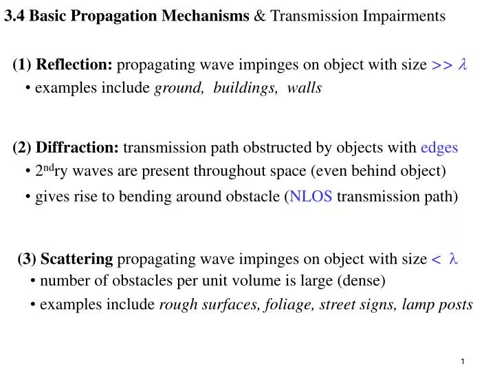
3.4 Basic Propagation Mechanisms & Transmission Impairments . (1) Reflection: propagating wave impinges on object with size >> examples include ground, buildings, walls. (2) Diffraction: transmission path obstructed by objects with edges

E N D
3.4 Basic Propagation Mechanisms & Transmission Impairments • (1) Reflection: propagating wave impinges on object with size >> • examples include ground, buildings, walls • (2) Diffraction: transmission path obstructed by objects with edges • 2ndry waves are present throughout space (even behind object) • gives rise to bending around obstacle (NLOS transmission path) • (3) Scattering propagating wave impinges on object with size < • number of obstacles per unit volume is large (dense) • examples include rough surfaces, foliage, street signs, lamp posts
at high frequencies diffraction & reflections depend on • geometry of objects • EM wave’s, amplitude, phase, & polarization at point of intersection • Models are used to predict received power or path loss (reciprocal) • based on refraction, reflection, scattering • Large Scale Models • Fading Models
3.5 Reflection: EM wave in 1st medium impinges on 2nd medium • part of the wave is transmitted • part of the wave is reflected • (1) plane-wave incident on a perfect dielectric(non-conductor) • part of energy is transmitted (refracted) into 2nd medium • part of energy is transmitted (reflected) back into 1st medium • assumes no loss of energy from absorption (not practically) • (2) plane-wave incident on a perfect conductor • all energy is reflected back into the medium • assumes no loss of energy from absorption (not practically)
incident wave reflected wave refracted wave boundary between dielectrics (reflecting surface) • (3) = Fersnel reflection coefficient relates Electric Field intensity • of reflected & refracted waves to incident wave as a function of: • material properties, • polarization of wave • angle of incidence • signal frequency
E|| E • (4) Polarization:EM waves are generally polarized • instantaneous electric field components are inorthogonal directions • in space represented as either: • (i) sum of 2 spatially orthogonal components (e.g. vertical • & horizontal) • (ii) left-handed or right handed circularly polarized components • reflected fieldsfrom a reflecting surface can be computed using • superposition for any arbitrary polarization
plane of incidence reflecting surface= boundary between dielectrics i r t • 3.5.1 Reflection from Dielectrics • assume no loss of energy from absorption • EM wave with E-fieldincident at i with boundary between 2 dielectric media • some energy is reflected into 1st media at r • remaining energy is refracted into 2nd media at t • reflections vary with the polarization of the E-field plane of incidence = plane containing incident, reflected, & refracted rays
Evi plane of incidence Ehi i r boundary between dielectrics (reflecting surface) t • Two distinct cases are used to study arbitrary directions of polarization • (1) Vertical Polarization: (Evi) E-field polarization is • parallelto theplane of incidence • normal component to reflecting surface • (2) Horizontal Polarization: (Ehi) E-field polarization is • perpendicular to the plane of incidence • parallel component to reflecting surface
i r t i r t Ei Er Hr Er Ei Hi 1,1, 1 Hi Hr 1,1, 1 2,2, 2 2,2, 2 Et Et Vertical Polarization: E-field in the plane of incidence Horizontal Polarization: E-field normal to plane of incidence • Ei & Hi = Incident electric and magnetic fields • Er& Hr = Reflected electric and magnetic fields • Et = Transmitted (penetrating)electric field
dielectric constant for perfect dielectric (e.g. perfect reflector of lossless material) given by • 0= 8.85 10-12 F/m • (1) EM Parameters of Materials • = permittivity (dielectric constant): measure of a materials ability • to resist current flow • = permeability: ratio of magnetic induction to magnetic field • intensity • = conductance: ability of a material to conduct electricity, • measured in Ω-1
highly conductive materials • r& are generally insensitive to operating frequency lossy dielectricmaterials will absorb power permittivity described with complex dielectric constant = 0 r -j’ (3.17) (3.18) where ’ = often permittivity of a material, is related to relative permittivityr = 0 r • 0 and r are generally constant • may be sensitive to operating frequency
(2) Reflections, Polarized Components & Fresnel Reflection • Coefficients • because of superposition – only 2 orthogonal polarizations need be • considered to solve general reflection problem • Maxwell’s Equationboundary conditions used to derive (3.19-3.23) • Fresnel reflection coefficientsfor E-field polarization at reflecting • surface boundary • ||represents coefficient for || E-field polarization • represents coefficient for E-field polarization
(i) E-field in plane of incidence (vertical polarization) || = (3.19) (ii) E-field not in plane of incidence (horizontal polarization) = (3.20) • i = intrinsic impedance of the ith medium • ratio of electric field to magnetic field for uniform plane wave in • ith medium • given by i= Fersnel reflection coefficients given by
velocity of an EM wave given by (3.21) i = r (3.22) Er = Ei (3.23a) Et = (1 + )Ei (3.23b) boundary conditionsat surface of incidence obey Snell’s Law • is either || or depending on polarization • | | 1 for a perfect conductor, wave is fully reflected • | | 0 for a lossy material, wave is fully refracted
||= (3.24) = (3.25) Simplification of reflection coefficients for vertical and horizontal polarization assuming: • radio wave propagating in free space (1st medium is free space) • 1 = 2 • Elliptically Polarized Waves have both vertical & horizontal components • waves can be depolarized (broken down) into vertical & horizontal • E-field components • superposition can be used to determine transmitted & reflected • waves
spatial vertical axis || orthogonal components of propagating wave spatial horizontal axis • (3) General Case ofreflection or transmission • horizontal & vertical axes of spatial coordinates may not coincide • with || & axes of propagating waves • for wave propagating out of the page define angle • measured counter clock-wise from horizontal axes
vertical & horizontal polarized components components perpendicular & parallel to plane of incidence EiH , EiV EdH, EdV (3.26) relationship of vertical & horizontal field components at the dielectric boundary EdH,EdVEiH , EiV= Time Varying Components of E-field • EdH, EdV= depolarized field components along the horizontal & • vertical axes • EiH , EiV= horizontal & vertical polarized components of incident • wave - E-field components may be represented by phasors
R = transformation matrix that maps E-field components , = angle between two sets of axes R = DC= depolarization matrix DC= • for case of reflection: • D= • D|| ||= || • for case of refraction (transmission): • D= 1+ • D|| ||= 1+ ||
1.0 0.8 0.6 0.4 0.2 0.0 |||| r=12 r=4 vertical polarization (E-field in plane of incidence) 0 10 20 30 40 50 60 70 80 90 Brewster Angle (B) for r=12 angle of incidence (i) Plot of Reflection Coefficients for Parallel Polarization for r= 12, 4 for i < B: a larger dielectric constant smaller || & smaller Er for i > B: a larger dielectric constant larger || & larger Er
|| 1.0 0.9 0.8 0.7 0.6 0.5 0.4 0.3 r=12 horizontal polarization (E-field not in plane of incidence) r=4 0 10 20 30 40 50 60 70 80 90 angle of incidence (i) Plot of Reflection Coefficients for Perpendicular Polarization for r= 12, 4 for given i: larger dielectric constant larger and larger Er
||= = • e.g. let medium 1 = free space & medium 2 = dielectric • if i 0o (wave is parallel to ground) • thenindependent of r, coefficients || 1 and |||| 1 • thus, if incident wave grazes the earth • ground may be modeled as a perfect reflector with || = 1 • regardless of polarization or ground dielectric properties • horizontal polarization results in 180 phase shift
B satisfies sin(B) = (3.27) • if 1st medium = free space & 2nd medium has relative permittivity r • then (3.27) can be expressed as sin(B) = (3.28) 3.5.2 Brewster Angle = B • Brewster angle only occurs for vertical (parallel) polarization • angle at which no reflection occurs in medium of origin • occurs when incident angle iis such that || = 0 i = B
Let r = 15 = 0.25 sin(B) = Let r = 4 B= sin-1(0.25) = 14.5o = 0.44 sin(B) = B= sin-1(0.44) = 26.6o e.g. 1st medium = free space
3.6 Ground Reflection – 2 Ray Model • Free Space Propagation model is inaccuratefor most mobile RF • channels • 2 Ray Ground Reflection model considers both LOS path & ground • reflected path • based on geometric optics • reasonably accurate for predicting large scale signal strength for • distances of several km • useful for • - mobile RF systems which use tall towers (> 50m) • - LOS microcell channels in urban environments • Assume • maximum LOS distances d 10km • earth is flat
ELOS Ei Er = Eg d E(d,t) = (3.33) i 0 (1) Determine Total Received E-field (in V/m) ETOT ETOT is combination of ELOS & Eg • ELOS= E-field of LOS component • Eg= E-field of ground reflected component • θi = θr LetE0= free space E-field (V/m) at distance d0 • Propagating Free Space E-field at distance d > d0 is given by • E-field’s envelope at distance d from transmitter given by • |E(d,t)| = E0 d0/d
Eg(d”,t) = (3.35) d’ ELOS Ei ht Eg d” h r i 0 d E-field for LOS and reflected wave relative to E0 given by: ELOS(d’,t) = (3.34) and ETOT = ELOS + Eg • assumes LOS & reflected waves arrive at the receiver with • - d’ = distance of LOS wave • - d” = distance of reflected wave
i = 0 Eg = Ei Et = (1+) Ei (3.36) (3.37a) (3.37b) ELOS d’ Ei Eg d” Et i 0 From laws of reflection in dielectrics (section 3.5.1) = reflection coefficient for ground
resultant E-field is vector sum of ELOS and Eg • total E-field Envelope is given by |ETOT| = |ELOS + Eg| (3.38) • total electric field given by ETOT(d,t) = (3.39) • Assume • i. perfect horizontal E-field Polarization • ii. perfect ground reflection • iii. small i (grazing incidence) ≈ -1 & Et ≈ 0 • reflected wave & incident wave haveequal magnitude • reflected wave is 180oout of phase with incident wave • transmitted wave≈ 0
= (3-40) ELOS h d’ Eg Ei ht h r d” 0 i ht +hr if d >> hr + ht Taylor series approximations yields (from 3-40) d (3-41) (2) Compute Phase Difference & Delay Between Two Components • path difference = d” – d’ determined from method of images
= (3-42) 0 π 2π d = (3-43) Δ if Δ = /n = 2π/n • time delay (3.44) once is known we can compute • phase difference • As d becomes large = d”-d’ becomes small • amplitudes of ELOS & Eg are nearly identical & differ only in phase
reflected path arrives at receiver at t = d”/c = = (3) Evaluate E-field when reflected path arrives at receiver ETOT(d,t)|t=d”/c = (3.45)
|ETOT(d)|= ETOT = (3.46) = (3.47) (3.48) = (4) Determine exact E-field for 2-ray ground model at distance d Use phasor diagram to find resultant E-field from combined direct & ground reflected rays:
-50 -60 -70 -80 -90 -100 -110 -120 -130 -140 fc = 3GHz fc = 7GHz fc = 11GHz Propagation Lossht = hr = 1, Gt = Gr = 0dB 101 102 103 104 m • As d increases ETOT(d) decreases in oscillatory manner • local maxima 6dB > free space value • local minima ≈ - dB (cancellation) • once d is large enough θΔ< π & ETOT(d) falls off asymtotically • with increasing d
this implies (3.50) V/m ETOT(d) (3.51) |ETOT(d)| For phase difference, < 0.6 radians (34o)sin(0.5 ) (3.49) d > if d satisfies 3.50 total E-fieldcan be approximated as: kis a constant related to E0 ht,hr, and e.g. at 900MHz if < 0.03m total E-field decays with d2
Pr(d) = (3.52a) Pr(d) = (3.52b) • received power falls off at 40dB/decade • receive power & path loss become independent of frequency if d >> Received Power at d is related to square of E-field by 3.2, 3.15, & 3.51
PL = PL(dB) = 40log d - (10logGt+ 10logGr + 20log ht + 20 log hr) (3.53) Path Loss for 2-ray model with antenna gains is expressed as: • 3.50 must hold • for short Tx-Rx distances use (3.39) to computetotal E field • evaluate (3.42) for = (180o) d = 4hthr/is where the ground • appears in 1stFresnel Zone between Tx & Rx • - 1st Fresnel distance zone is useful parameter in microcell path • loss models


![G3 - RADIO WAVE PROPAGATION [3 Exam Questions -- 3 Groups]](https://cdn0.slideserve.com/819386/g3-radio-wave-propagation-3-exam-questions-3-groups-dt.jpg)