Download
1 / 17
170 likes | 288 Views
Noise of hot electrons in anisotropic semiconductors in the presence of a magnetic field. Francesco Ciccarello in collaboration with: S. Zammito and M. Zarcone CNISM & Dipartimento di Fisica e Tecnologie Relative, University of Palermo (Italy).

E N D
Noise of hot electrons in anisotropic semiconductors in the presence of a magnetic field Francesco Ciccarello in collaboration with: S. Zammito and M. Zarcone CNISM & Dipartimento di Fisica e Tecnologie Relative, University of Palermo (Italy) UPON 2008, École Normale Supérieure de Lyon (France), June 2–6, 2008
a sketch of this work problem in an anisotropic seminconductor: how hot-electron velocity fluctuations are affected by the presence of a static magnetic field? ouroutcomes 1. the relative importance of noise can be reduced 2. partition noise can be strongly attenuated 3. a simultaneous increase of conductivity can take place
conduction band of Si 3 pairsofenergetically-equivalent ellipsoidalvalleysalong: <100> (“valleys 1” ) <010> (“valleys 2” ) <001> (“valleys 3” ) ml=0.916 m0 > mt=0.19 m0 electrons’ inertia does depend on the direction and valleys
we apply an intense electric field (~ kV/cm) valleys 1 cold& lesspopulated valleys 2,3 hot& mostpopulated
velocity fluctuations heavyvalleys 1 slow electrons light valleys 2,3 fastelectrons v1x< v2x,v3x v1x < vd < v2x=v3x longitudinal velocity autocorrelation function partitionnoise in the <100> case
let us add a magnetic field in a Hall-geometry <001> B EH EA <010> B=0B≠0 valleys1 cold& mostpopulatedhot & lesspopulated valleys 2,3 hot& lesspopulatedcold& mostpopulated also: conductivity is enhanced Asche M and Sarbei O G, Phys. Stat. Sol. 37, 439 (1970) Asche M et al., Phys. Stat. Sol. (b) 60, 497 (1973)
how are velocity fluctuations affected? n-GaAs (isotropic) Ciccarello F and Zarcone M, J. Appl. Phys. 99,113702 (2006) Ciccarello F and Zarcone, AIP Conf. Proc. 800, 492 (2005 ) Ciccarello F and Zarcone, AIP Conf. Proc. 780, 159 (2005 )
our Monte Carlo approach free-flight Newtonian equation scattering processes 3 f -type intervalley processes 3 g -type intravalley processes acoustic scattering (valley i j) (valley i i) Brunetti R, et al., J. Appl. Phys. 52, 6713 (1981) Jacoboni C, Minder R and Majni ,J. Chem. Phys. Solids 36,1129 (1975) Hall field we iteratively look for EHsuch that Raguotis R A, Repsas K K and Tauras V K, Lith. J. Phys. 31, 213 (1991) Raguotis R, Phys. Stat. Sol. (b) 174 K67 (1992) regime T=77 K; stationary conditions; maximum magnetic-field strengths allowing magnetic-field effects competing with electric-field ones
central result velocity variance drift velocity EA=10 kV/cm EA=10 kV/cm EA=6 kV/cm EA=6 kV/cm average energy standard deviation/drift velocity EA=10 kV/cm EA=10 kV/cm ~20~% EA=6 kV/cm EA=6 kV/cm the magnetic-field action yields a more intense & cleaner current
insight into the mechanism behind valley average energies valley occupation probabilities valley average velocities EA=6 kV/cm EA=6 kV/cm valleys 2, 3 valleys 1 valleys 2, 3 drift velocity EA=6 kV/cm mean valleys 2, 3 valleys 1 valleys 1 the magnetic field increases population of high-velocity valleys
isotropic case: free-flight motion A. D. Boardman et al., Phys. Stat. Sol. (a), 4, 133 (1971) cyclotron frequency center magnitude measures the maximum amount of gainable energy
K*-space Herring-Vogt transformation Herring C and Vogt E, Phys. Rev. 101, 944 (1956) dispersion law in each valley velocity vs. wavevector nonparabolicity effects
fields* free-flight equation in each valley isotropic in k *-space fields are valley-dependent as B grows the effect of EH becomes more & more significant measures the maximum energy that can be gained
fields* valleys 1 valleys 2 valleys 3
autocorrelation functions longitudinal B=0 vs. B=4.5 T EA=5 kV/cm partition-noise attenuation is partition noise lost? transversal average velocity longitudinal vs. transversal partition-noise is shifted towards the transversal direction EA=5 kV/cm B=4.5 T valleys 1 valleys 3 different valleys have different transversal velocities valleys 2
conclusions ∙B can give rise to a more ordered conductive state with: - higher mobility - reduced importance of fluctuations - attenuated partition noise - moderate electron heating
open questions & outlook ∙ what about different Hall geometries such as EA ll <011> & B ll <100> or EA ll <111> & B ll <110>?? ∙ what’s the optimal geometry in order to minimize noise? ∙ is there a statistical procedure able to filter out mere fluctuations from cyclotronic oscillations? ∙ is there a better system able to exhibit such phenomena (if possible, at room temperature)? ∙ noise spectrum analysis thanksforyourattention!