Compensators (Dorf & Bishop)

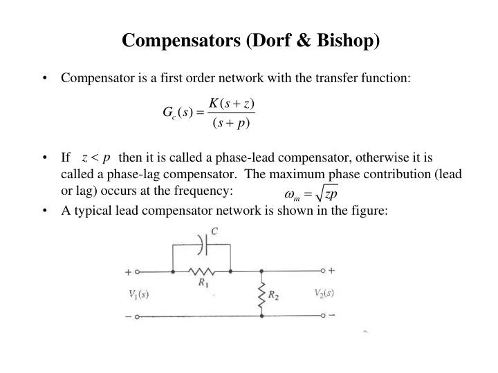
1. Compensators (Dorf & Bishop) • Compensator is a first order network with the transfer function: • If then it is called a phase-lead compensator, otherwise it is called a phase-lag compensator. The maximum phase contribution (lead or lag) occurs at the frequency: • A typical lead compensator network is shown in the figure:

2. The transfer function of the above lead compensator network can be easily shown to be: • A typical lag compensator network is shown in the figure:

3. The transfer function of the above lag compensator network can be easily shown to be:

4. Lead Design Using Root Locus (Dorf & Bishop) • The design is based on reshaping the root locus by adding a pole and a zero to the open-loop transfer function to force the root locus to pass through a desired closed-loop pole location. The steps involved are: • Determine the desired closed-loop pole location from the given specification. • Draw the root locus for the uncompensated system and check whether the desired pole location can be achieved by varying the gain alone. • If a compensator is necessary, place the zero of the lead compensator directly below the desired pole location or to the left of first two real poles.

5. . Determine the lead compensator pole location so that the total angle at the desired pole location is 180 degrees. (Note that this follows from the angle criterion of the root locus). • Calculate the system gain at the desired pole location and check whether it satisfies the steady-state error requirements. If not change the desired pole location, and repeat the steps. Some Comments on Lead Compensators: • Lead compensators increases the relative stability by increasing the phase margin. Hence it is used to stabilize an unstable system. • Lead compensator is used when the system is unstable for all values of gain or when the system is stable with undesirable transient response characteristics.

6. Example 1 (Dorf and Bishop) • Consider a second-order system given by: • Design a lead compensator so that cascade compensated system satisfies: • Settling time (with a 2% criterion) of less than or equal to 4 seconds • Percentage overshoot of less than or equal to 35%. • To satisfy the percentage overshoot requirements, the damping factor should satisfy: • To satisfy the settling time requirement, we have: Or • If we choose

7. We place the zero of the lead compensator directly below the desired pole location, or • The angle at the desired pole location: • If the desired pole location has to lie on the root locus, then the angle from the undetermined pole should be: • We then draw a line at 38 degrees to real axis and intersection the desired pole location as shown in the figure. The compensator pole location is given by the point at which this line intersects the real axis. • Therefore compensator pole is given by • The lead compensator is given by: • The compensated transfer function of the system is given by • The gain evaluated using the magnitude criterion is

8. .

9. Lag Design Using Root Locus (Ogata) • Lag compensator is used when system meets stability requirements but does not satisfy the steady-state error specifications. • Lag compensator introduces a phase lag and hence can destabilize the system. • Lag compensators are never used when the system is unstable or when the system has low stability margin. The step involved in lag design are: • Draw the root locus of the uncompensated system. • Determine the desired pole location from the transient response specifications.

10. Determine the loop gain at the desired pole location and the steady state error constant. • Calculate the increase in the static error constant required to satisfy the specifications. • Choose the pole and zero locations of the lag compensator that produce the required increase in the particular static error constant without significantly changing the original root locus. • Note that to satisfy the requirements in the above step, the pole and zero locations are chosen close to one another but yet maintaining the ratio required to fulfill the static error specifications. • Draw a new root locus corresponding to the compensated system and check whether it meets all the specifications.

11. Example 2 (Dorf & Bishop) • Consider a second order system given by: • We require damping ratio of the dominant closed-loop poles to be 0.45 and a static velocity error constant equal to 20. To satisfy these specifications, we design a lag compensator. • The root locus of the uncompensated system is shown in the figure on the left. Drawing a line corresponding to the damping factor of 0.45, gives us the dominant pole locations: • Calculating the gain at the desired pole location, we have K=5 (use magnitude criterion). • The velocity error constant of the uncompensated system is • The required zero to pole ratio of lag compensator is given by 20/2.5=8.

12. Choosing both zero and pole close to the origin, we have • The compensated system transfer function is given by: • The root locus for the compensated system is shown in the figure on the right.

13. Proportional-Integral-Derivative Control • Proportional-Integral-Derivative (PID) controllers are very popular in the process control industry. • They can be easily tuned to achieve good closed-loop performance using simple rules. • PID controller can take many forms: PD controller when integral constant is set to zero, or PI controller when derivative constant is set to zero, or just P controller when integral and derivative constants are both set to zero. • Ziegler-Nichols Method: In this method, by setting integral and derivative constants to zero, the proportional gain is increased till the system just oscillates. The various constants are calculated as follows:

14. .

15. Note that Ziegler-Nichols method of tuning PID controllers does not design to any specification. However, it well known to provide “good” behaviour for process controllers. • Note that in practice, we never build a pure differentiator, due noise problems inherent in such a device. Therefore, the derivative term is always implemented with pole in addition to the zero at the origin. PD control is often realized with a sensor that can measure directly the derivative of the output, e.g., tachometer.

16. Fixed Structure Compensators (Stefani) • Consider a unity feedback cascaded compensated system shown. If

17. A fixed structure compensator has a fixed form and dimension regardless of the application. • These compensators can place a small number of closed loop poles at desired locations. • If a closed-loop system is of order n and there are m (where m<n) multiplying factors in the compensator, then m closed-loop poles can be placed at arbitrarily chosen locations. • The m multiplying factors can be obtained by equating the closed-loop characteristic polynomial to the desired characteristic polynomial (which can be calculated from the desired pole locations). • The equation used to calculate the multiplying factors are always linear and may possibly be simultaneous. • PID controller is an example of a fixed-structure compensator. • These compensators are also known as pole-placement compensators.

18. Example 3 (Stefani) • Consider a second-order plant given by • Design a PID Compensator such that the closed-loop poles of the unity feedback cascaded compensated system are at s=-3, s=-4, and s=-20. Solution: • The desired closed-loop characteristic polynomial is given by: • The actual closed-loop characteristic polynomial is given by: • Equating the coefficients the like powers of s in the two polynomials we have

19. . • PID compensator is given by

20. References • J.H. DiStefano, A.R. Stubberud, I.J. Williams, Feedback and Control Systems, Schaum’s Outline Series, McGraw Hill, Singapore, 1987. • M .Ogata, Modern Control Engineering, Fourth edition, Prentice-Hall Inc, NJ, 2002. • Y.H. Leung, System Theory 318 Notes, 2002. • R.C. Dorf and R.H. Bishop, Modern Control Systems, Prentice-Hall Inc., 8th or 9th edition. • A. Stefani, Savant, Shahian, and Hostetter, Design of Feedback Control Systems, Saunders College Publishing, U.S.A, 1994.