Download
1 / 31
310 likes | 452 Views
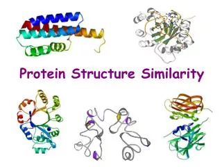
Approximation of Protein Structure for Fast Similarity Measures. Itay Lotan Fabian Schwarzer. Comparing Protein Structures. Same protein:. vs. Analysis of MDS and MCS trajectories. Graph-based Methods. Structure prediction applications. Evaluating decoy sets

E N D
Approximation of Protein Structure for Fast Similarity Measures Itay Lotan Fabian Schwarzer
Comparing Protein Structures Same protein: vs. Analysis of MDS and MCStrajectories Graph-based Methods Structure prediction applications • Evaluating decoy sets • Clustering predictions (Shortle et al, Biophysics ’98) Stochastic Roadmap Simulation(Apaydin et al, RECOMB ’02) http://folding.stanford.edu
k Nearest-Neighbors Problem Given a set S of conformations of a protein and a query conformation c, find the k conformations in S most similar to c. Can be done in N– size of S L – time to compare two conformations
k Nearest-Neighbors Problem What if needed for all cin S? -too much time • Can be improved by: • Reducing L • A more efficient algorithm
Our Solution Reduce structure description Approximate but fast similarity measures Reduce description further Efficient nearest-neighbor algorithms can be used
Description of a Protein’s Structure 3n coordinates of Cα atoms (n – Number of residues)
m-Averaged Approximation • Cut chain into pieces of length m • Replace each sequence of m Cα atoms by its centroid 3n coordinates 3n/m coordinates
Similarity Measures - cRMS The RMS of the distances between corresponding atoms after the two conformations are optimally aligned Computed in O(n) time
Similarity Measures - dRMS The Euclidean distance between the intra-molecular distances matrices of the two conformations Computed in O(n2) time
Evaluation: Test Sets • Decoy sets: conformations from the Park-Levitt set (Park et al, JMB ’97), N =10,000 • Random sets: conformations generated by the program FOLDTRAJ (Feldman & Hogue, Proteins ’00),N = 5000 8 structurally diverse proteins of size 54 -76 residues:
dRMS m cRMS 3 4 6 9 12 Decoy Sets Correlation 0.99 0.96 – 0.98 0.98 – 0.99 0.94 – 0.97 0.92 – 0.99 0.78 – 0.93 0.81 – 0.98 0.65 – 0.96 0.54 – 0.92 0.52 – 0.69 Higher Correlation for random sets!
Speed-up for Decoy Sets • 9x for cRMS (m = 9) • 36x for dRMS (m = 6) with very small error For random sets the speed-up for dRMS goes up to 81x (m = 9)
Efficient Nearest-Neighbor Algorithms There are efficient nearest-neighbor algorithms, but they are not compatible with similarity measures: cRMS is not a Euclidean metric dRMS uses a space of dimensionality n(n-1)/2
Further Dimensionality Reduction of dRMS kd-trees require dimension 20 m-averaging with dRMS is not enough Reduce further using SVD SVD: A tool for principal component analysis. Computes directions of greatest variance.
Reduction Using SVD • Stack m-averaged distance matrices as vectors • Compute the SVD of entire set • Project onto most important singular vectors dRMS is thus reduced to 20 dimensions Without m-averaging SVD can be too costly
Testing the Method • Use decoy sets (N = 10,000) and random sets (N = 5,000) • m-averaging with (m = 4) • Project onto 16 PCs for decoys, 12 PCs for random sets • Find k = 10, 25, 100 NNs for 250 conformations in each set
Results • Decoy sets: • ~77% correct • Furthest approximate NN off by 10% - 15% • ~4k approximate NNs contain all true k NNs • Random sets: • 71%, 76%, 84% correct respectively • Furthest approximate NN off by 5% - 10% • ~3k approximate NNs contain all true k NNs
More Results: N = 100,000 • 1CTF decoys: • ~70% correct • Furthest approximate NN off by ~20% • ~6k approximate NNs contain all true k NNs • 1CTF random: • 46%, 48%, 60% correct respectively • Furthest approximate NN off by ~16% • ~7k approximate NNs contain all true k NNs
Running Time N = 100,000, m=4, PC = 16 Find k = 100 for each conformation Brute-force: ~84 hours Brute-force + m-averaging: ~4.8 hours Brute-force + m-averaging + SVD: 41 minutes Kd-tree + m-averaging + SVD: 19 minutes kd-trees will have more impact for larger sets
Structural Classification Computing the similarity between structures of two different proteins is more involved: 2MM1 1IRD vs. The correspondence problem: Which parts of the two structures should be compared?
STRUCTAL (Subbiah et al, ’93) • Compute optimal correspondence using dynamic programming • Optimally align the corresponding parts in space to minimize cRMS • Repeat until convergence O(n1n2) time
STRUCTAL + m-averaging • 256 protein domains (180 – 420 res) • 3691 good matches (Sandelin’s PROTOFARM) • 6375 random pairs • Compute SAS scores (cRMS/length*100) m correlation speed-up 3 0.81 ~9x 0.77 ~16x 4 5 0.70 ~25x
OK (P < 0.005) BAD (P > 0.005) Number of pairs SAS score
Random Chains c5 c7 • The dimensions are uncorrelated • Average behavior can be approximated by normal variables: c2 c6 c8 cn-1 c0 c4 c1 c3
1-D Haar Wavelet Transform Recursive averaging and differencing of the values Detail Coefficients Level Averages [ 9 7 2 6 5 1 4 6 ] 3 2 [ 8 4 3 5 ] [ 1 -2 2 -1 ] 1 [ 6 4 ] [ -2 -1 ] 0 [ 1 ] [ 5 ] [ 9 7 2 6 5 1 4 6 ] [ 5 1 -2 -11 -2 2 1]
Transform of Random Chains • pdf of the detail coefficients is: • Coefficients expected to be ordered! • Discard coefficients starting at lowest level Discarding lowest levels of detail coeeficients m-averaging
Random Chains and Proteins • Protein backbones behave on average like random chains • Chain topology • Limited compactness
Conclusion • Fast computation of similarity measures • Trade-off between speed and precision • Exploits chain topology of proteins and limited compactness • Allows use of efficient nearest-neighbor algorithms • Can be used as filter when precision is important