Download
1 / 29
290 likes | 416 Views
Characterization of short pulses . A. Yartsev. What is good to know about short pulses?. Energy of each pulse Average power Spectrum Spatial distribution Temporal profile Satellites Duration Shape . Energy/Power measurements. fro m pico-Joule to peta-Watt. Physics of detection

E N D
Characterization of short pulses. A. Yartsev
What is good to know about short pulses? • Energy of each pulse • Average power • Spectrum • Spatial distribution • Temporal profile • Satellites • Duration • Shape
Energy/Power measurements.from pico-Joule to peta-Watt • Physics of detection • Choice of detector • Linearity • Sensitivity • Spectral response • Response time • Damage
Spectral shape • What do you need the spectrum for? • Sensitivity range. • Calibration of the spectrometer. • Dynamic range. • Optics on the way. • Fibber ”wave guides”.
Beam profile • Assume Gaussian? • Measure power through calibrated pinholes • Blade-edge method • Measure real profile. • 2-D detector: CCD matrix • 1-D array detector • Linearity of response
Temporal profile:What for? • Satellites: quality of amplification, quality of measurements • Pulse duration: FWHM • Instrumental response function • Transform-limited pulse • Pulses of random shape
Electrical (direct) measurements of pulse duration: not fast enough and (very) expensive. • Photodiode: >10 ps (+fast Oscilloscope) • Streak Camera: 100 fs (?), ~1 ps
All-optical methods • Time from distance: 1 fs 0.3 m • Math: correlation function • determines F(t) if G() is measured and F’(t) is known.
Autocorrelation • Interferometric AC • Intensity AC • Single – shot AC • Both F(t) and F’(t) are replica’s of the same function E(t)exp
Interferometric AC • F(t) = E(t)exc[it+i(t)] • I1() =|E(t)exc[it+i(t)] +E(t-)exc[i(t- )+i(t-)]|2dt • I2() =|{E(t)exc[it+i(t)] +E(t-)exc[i(t- )+i(t-)]}2|2dt • First order AC: I1(=0)/I1() = 2 • Second order AC: I2(=0)/I2() = 8
Limitions of AC • Non-specific: one has assume a particular pulse shape. • Returns only amplitude.
Full-field characterization of femtosecond pulses by spectrumand cross-correlation measurements OPTICS LETTERS / Vol. 24, No. 23 / December 1, 1999 J. W. Nicholson, J. Jasapara, and W. Rudolph F. G. Omenetto and A. J. Taylor
Frequennsy-resolved optical gating FROG Rev. Sci. Instrum., Vol. 68, No. 9, September 1997 R. Trebino, K. W. DeLong, D. N. Fittinghoff, J. N. Sweetser,
Rev. Sci. Instrum., Vol. 68, No. 9, September 1997 R. Trebino, K. W. DeLong, D. N. Fittinghoff, J. N. Sweetser, FROG
Limitions of FROG • Requirements on set-up: linear detector response, step size, S/N. • Delay-scanning technique. • Measures 2D characteristic – long. • Non-specific: needs a (complicated) retrival to get pulse. • Does not always converge.
X-FROG:spectrally-resolved cross-correlation of an unknown pulse with the reference pulse.
TADPOLE Rev. Sci. Instrum., Vol. 68, No. 9, September 1997 R. Trebino, K. W. DeLong, D. N. Fittinghoff, J. N. Sweetser,
FRPP: pump-probe FROG OPTICS LETTERS / Vol. 27, No. 13 / July 1, 2002 S. Yeremenko, A. Baltuˇska, F. de Haan, M. S. Pshenichnikov, D. A. Wiersma
Self-Referencing Spectral Interferometry for Measuring Ultrashort Optical Pulses SPIDER IEEE J Quant.Elctr. Vol. 35, No. 4, April 1999 C. Iaconis, I.A. Walmsley
Advantages of SPIDER • No moving parts • Direct reconstruction (>1kHz) • Noise immunity • Low sensitivity to detector spectral response • Precision and consistency mesures from data
Limitions of SPIDER • Has to be optimised for a particular time-and spectral range. • Requires calibration. • Very sensitive to delay between pulses – sensitive to alignment.
After SPIDER: SEA-SPIDER E. M. Kosik and A. S. Radunsky I. A. Walmsley C. Dorrer OPTICS LETTERS Vol. 30, No. 3, 2005
After SPIDER: 2DSI OPTICS LETTERS / Vol. 31, No. 13 / July 1, 2006 J. R. Birge, R. Ell, F. X. Kärtner