Download
1 / 17
180 likes | 332 Views
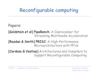
Reconfigurable Computing (EN2911X, Fall07) Lecture 05: Verilog (1/3). Prof. Sherief Reda Division of Engineering, Brown University http://ic.engin.brown.edu. Introduction to Verilog. Why are the advantages of Hardware Definition Languages? Verilog is a HDL similar in syntax to C

E N D
Reconfigurable Computing (EN2911X, Fall07) Lecture 05: Verilog (1/3) Prof. Sherief Reda Division of Engineering, Brown University http://ic.engin.brown.edu
Introduction to Verilog • Why are the advantages of Hardware Definition Languages? • Verilog is a HDL similar in syntax to C • Verilog is case sensitive • Many online textbooks available from Brown library • Verilog digital system design • Verilog quickstart • The Verilog hardware description language • Lecture examples from “Verilog HDL” by S. Palnitkar
Verilog modules module toggle(q, clk, reset); … <functionality of module> … endmodule toggle reset q clk • The internal of each module can be defined at four level of abstraction • Behavioral or algorithmic level • Dataflow level • Gate level • Switch level • Verilog allows different levels of abstraction to be mixed in the same module.
Basic concepts • Comments are designated by // to the end of a line or by /* to */ across several lines. • Number specification. <size>’<base format><number> specifies the number of bits in the number d or D for decimal h or H for hexadecimal b or B for binary o or O for octal Number depends on the base • Examples: • 4’b1111 • 12’habc • 16’d235 • 12’h13x • -6’d3 • 12’b1111_0000_1010 X or x: don’t care Z or z: high impedence _ : used for readability
Data types • Nets represent connections between hardware elements. They are continuously driven by output of connected devices. They are declared using the keyword wire. • wire a; • wire b, c; • wire d=1’b0; • Registers represent data storage elements. They retain value until another value is placed onto them. In Verilog, a register is merely a variable that can hold a value. They do not need a clock as hardware registers do. • reg reset; • initial • begin • reset = 1’b1; • #100 reset=1’b0; • end
Data types • A net or register can be declared as vectors. Example of declarations: • wire a; • wire [7:0] bus; • wire [31:0] busA, busB, busC; • reg clock; • reg [0:40] virt_address; • It is possible to address bits or parts of vectors • busA[7] • bus[2:0] • virt_addr[0:2] • Use integer for counting. Example. • integer counter • initial • counter = -1;
Data types • Reals • real delta; • initial • begin • delta = 4e10; • delta = 2.13; • end • integer i; • initial • i = delta; • Arrays. It is possible to have arrays of type reg, integer, real • integer count[0:7]; • reg [4:0] port_id[0:7]; • integer matrix[4:0][0:255];
Data types • Memories. Used to model register files, RAMs and ROMs. Modeled in Verilog as a one-dimensional array of registers. Examples. • reg mem1bit[0:1023]; • reg [7:0] membyte[0:1023]; • membyte[511]; • Parameters. Define constants and can’t be used as variables. • parameter port_id=5; • Strings can be stored in reg. The width of the register variables must be large enough to hold the string. • reg [8*19:1] string_value; • initial • string_value = “Hello Verilog World”;
Modules and ports module fulladd4(sum, c_out, a, b, c_in); output [3:0] sum; output c_out; input [3:0] a, b; input c_in; … … endmodule • All port declarations (input, output, inout) are implicitly declared as wire. • If the output hold their value, they must be declared are reg module DFF(q, d, clk, reset); output reg q; input d, clk, reset; … … endmodule
Module declaration (ANSI C style) module fulladd4(output reg[3:0] sum, output reg c_out, input [3:0] a, b, input c_in); … … endmodule
Module instantiation module Top; reg [3:0] A, B; reg C_IN; wire [3:0] SUM; wire C_OUT; // one way fulladd4 FA1(SUM, C_OUT, A, B, CIN); // another possible way fulladd4 FA2(.c_out(C_OUT), .sum(SUM), .b(B), .c_in(C_IN), .a(A)); … endmodule externally, inputs can be a reg or a wire; internally must be wires externally must be wires module fulladd4(sum, c_out, a, b, c_in); output [3:0] sum; output c_out; input [3:0] a, b; input c_in; … … endmodule
Gate level modeling (structural) . wire Z, Z1, OUT, OUT1, OUT2, IN1, IN2; and a1(OUT1, IN1, IN2); nand na1(OUT2, IN1, IN2); xor x1(OUT, OUT1, OUT2); not (Z, OUT); buf final (Z1, Z); . • All instances are executed concurrently just as in hardware • Instance name is not necessary • The first terminal in the list of terminals is an output and the other terminals are inputs • Not the most interesting modeling technique for our class
Array of gate instances wire [7:0] OUT, IN1, IN2; // array of gates instantiations nand n_gate [7:0] (OUT, IN1, IN2); // which is equivalent to the following nand n_gate0 (OUT[0], IN1[0], IN2[0]); nand n_gate1 (OUT[1], IN1[1], IN2[1]); nand n_gate2 (OUT[2], IN1[2], IN2[2]); nand n_gate3 (OUT[3], IN1[3], IN2[3]); nand n_gate4 (OUT[4], IN1[4], IN2[4]); nand n_gate5 (OUT[5], IN1[5], IN2[5]); nand n_gate6 (OUT[6], IN1[6], IN2[6]); nand n_gate7 (OUT[7], IN1[7], IN2[7]);
Dataflow modeling • Module is designed by specifying the data flow, where the designer is aware of how data flows between hardware registers and how the data is processed in the design • The continuous assignment is one of the main constructs used in dataflow modeling • assign out = i1 & i2; • assign addr[15:0] = addr1[15:0] ^ addr2[15:0]; • assign {c_out, sum[3:0]}=a[3:0]+b[3:0]+c_in; • A continuous assignment is always active and the assignment expression is evaluated as soon as one of the right-hand-side variables change • Left-hand side must be a scalar or vector net. Right-hand side operands can be registers, nets, integers, real, …
Operator types in dataflow expressions • Operators are similar to C except that there are no ++ or – • Arithmetic: *, /, +, -, % and ** • Logical: !, && and || • Relational: >, <, >= and <= • Equality: ==, !=, === and !== • Bitwise: ~, &, |, ^ and ^~ • Reduction: &, ~&, |, ~|, ^ and ^~ • Shift: <<, >>, >>> and <<< • Concatenation: { } • Replication: {{}} • Conditional: ?:
Example module mux4(out, i0, i1, i2, i3, s1, s0); output out; input i0, i1, i2, i3; output s1, s0; assign out = (~s1 & ~s0 & i0) | (~s1 & s0 & i1) | (s1 & ~s0 & i2) | (s1 & s0 & i3); // OR THIS WAY assign out = s1 ? (s0 ? i3:i2) : (s0 ? i1:i0); endmodule
Covered an introduction to Verilog Next time behavioral modeling Lab 0 is ready to warm up I will distribute lab 1 (game implementation) next time Summary