Download
1 / 22
220 likes | 368 Views
Domain Decomposed Parallel Heat Distribution Problem in Two Dimensions. Yana Kortsarts Jeff Rufinus Widener University Computer Science Department. Introduction.

E N D
Domain Decomposed Parallel Heat DistributionProblem in Two Dimensions Yana Kortsarts Jeff Rufinus Widener University Computer Science Department
Introduction • 2004: Office of Science in the Department of Energy issued a twenty-year strategic plan with seven highest priorities ranging from fusion energy to genomics. • To achieve the necessary levels of algorithmic and computational capabilities it is essential to educate students in computation and computational techniques. • Parallel Computing topic is one of the attractive topics in computation science field
Introductory Parallel Computer Course • Computer Science Department, Widener University, CS and CIS majors • Series of two courses Introduction to Parallel Computing I and II • Resources: computer cluster of six nodes, each node has two 2.4 GHz processors and 1 GB of memory, nodes are connected by Gigabit Ethernet switch.
Course Curriculum • Matrix Manipulation • Numerical Simulation Concepts: • Direct applications in science and engineering • Introduction to MPI libraries and their applications • Concepts of parallelism • Finite difference method for the 2-D heat equation using parallel algorithm
2-D Heat Distribution Problem The problem: to determine the temperature u(x,y,t) in an isotropic two-dimensional rectangular plate The model:
Finite Difference Method • The finite difference method begins with thediscretization of space and time such that there is an integer number of points in space and an integer number of times at which we calculate the temperature (xi , yj) tk tk+1 t y x
We will use the following notation: We will use the finite difference approximations for the derivatives: Expressing ui,j,k+1 from this equation yields:
Finite Difference Method Explicit Scheme ui,j+1,k ui-1,j,k ui,j,k ui+1,j,k ui,j,k+1 k k + 1 ui,j-1,k
Single Processor Implementation double u_old[n+1][n+1], u_new[n+1][n+1]; Initialize u_old with initial values and boundary conditions; while (still time points to compute) { for (i = 1; i < n; i++) { for (j = 1; j < n; j++) { compute u_new[i, j] using formula (1) }//end of for } // end of for u_old u_new; } // end of while
Parallel ImplementationDomain Decomposition • Dividing computation and data into pieces • Domain could be decomposed in three ways: • Column-wise: adjacent groups of columns (A) • Row-wise: adjacent groups of rows (B) • Block-wise: adjacent groups of two dimensional blocks (C)
Domain Decomposition and Partition Example: column-wise domain decomposition method, 200 points to be calculated simultaneously, 4 processors MPI_Send and MPI_Recv Processor 4 x149…x199 Processor 1 x0…x49 Processor 2 x50…x99 Processor3 x100…x149
Load Imbalance • When dividing the data into processes we have to pay attention to the number of loads being processed by each processor • Uneven load distribution may cause some processes to finish earlier than others • Load imbalance is one source of overhead • Good task mapping is needed • All tasks should be mapped onto processes as evenly as possible so that all tasks complete in the shortest amount of time and the idle time is minimized
Communication • Communication time depends on the latency and the speed of communication network – these two factors are much slower than CPU’s communication time • There is a catch of using too many communications
Running Time and Speedup • The running time of one time iteration of the sequential algorithm is(MN), where M and N are numbers of grid points in each direction • The running time of one time iteration of the parallel algorithm is: computational time + communication time = = (MN/p) + B where p is the number of processors and B is the total send-receive communication time that is required for one time iteration • The speedup is always defined as:
Results The temperature distribution on the two-dimensional plate at a much later time
Results • Two cases were considered: M x N = 1000 M x N = 500,000. • Next slide shows the speed-up versus the number of processors for two different inputs: 500,000 (the top chart) and 1000 (the bottom chart). • The dashed line indicates the speed-up equals to one, which is the sequential version of the algorithm. • The higher the speed-up (at a specific number of processors) means the better the performance of the parallel algorithm. • Most of the results come from the column-wise domain decomposition method.
Results • For the case of input= 1000, the sequential version (with p = 1) is faster than the parallel version (p ≥ 2). The parallel version is slower because of the latency and speed of the communication network which does not exist in the sequential version. • The top chart shows the speedup versus the number of processors for total input= 500,000. In this case, as we increase the number of processors, the speedup also increases, reaching the speedup of ~ 4.13 at p =10. • For a large number of inputs the communication time begins to catch up with the CPU’s computation time, resulting in a better performance of the parallel algorithm.
Speedup comparisons for column-wise and block-wise decomposition methods for number of processors equals to 4 and 9
Results • Overall, the speedups between the two methods are not very different. • For number of inputs = 1,000 the column-wise decomposition produces better speed-ups than the block-wise decomposition. • For number of inputs = 500,000, we have a mixed result. The column-wise method performs better for 9 processors while the block-wise method performs (slightly) better for 4 processors. • The results given in the table do not give a conclusive idea of which decomposition method is better, unless the number of inputs and the number of processors could be extended beyond the ones used in here.
Summary • Numerical simulation of two-dimensional heat distribution has been used as an example that can be used to teach parallel computing concepts in an introductory course. • With this simple example we introduce the core concepts of parallelism: • Domain decomposition and partitioning • Load balancing and mapping • Communication • Speedup • We show the benchmarking results of the parallel version of two-dimensional heat distribution problem with different number of processors.
References 1. J. Dongarra, I. Foster, G. Fox, W. Gropp, K. Kennedy, L. Torczon, and A. White, (Editors), Sourcebook of Parallel Computing. Elsevier Science (2003). 2. I. Foster, Designing and Building Parallel Programs. Addison Wesley (1994). 3. G. E. Karniadakis and R. M. Kirby, Parallel Scientific Computing in C++ and MPI. Cambridge University Press (2003). 4. M. J. Quinn, Parallel Programming in C with MPI and OpenMP. McGraw Hill Publishers (2005). 5. B. Wilkinson and M. Allen, Parallel Programming. Second edition. Prentice-Hall (2005). 6. M. Snir, S. Otto, S. Huss-Lederman, D. Walker and J. Dongarra, MPI The Complete Reference, Volume 1. Second edition. MIT Press (1998). 7. W. F. Ames, Numerical Methods for Partial Differential Equations. Second edition. Academic Press, New York (1977). 8. T. Myint-U and L. Debnath, Partial Differential Equations for Scientists and Engineers. Elsevier Science (1987). 9. G. D. Smith, Numerical Solution of Partial Differential Equations: Finite Difference Methods. Third edition. Oxford University Press (1985). 10. S. S. Rao, Applied Numerical Methods for Engineers and Scientists. Prentice-Hall (2002).