Download
1 / 22
230 likes | 575 Views
Performance Study of Domain Decomposed Parallel Matrix Vector Multiplication Programs. Yana Kortsarts Jeff Rufinus Widener University Computer Science Department. Introduction. Matrix computation is still one of many active areas of parallel numerical computing research.

E N D
Performance Study of Domain Decomposed Parallel Matrix Vector Multiplication Programs Yana Kortsarts Jeff Rufinus Widener University Computer Science Department
Introduction • Matrix computation is still one of many active areas of parallel numerical computing research. • There are many serial and parallel matrix computation algorithms discussed in the literature. Discussions on the parallel matrix-vector multiplication (MVM) algorithm are rare, except perhaps in some parallel computing textbooks • MVM problem is simple but computationally very rich. • The concepts of domain decomposition as well as communication between the processors are inherent in MVM. • MVM is an excellent example for exploring and learning the concept of parallelism. • MVM has applications in science and engineering.
The Problem and Sequential Algorithm • A – dense square matrix of size N x N • b is a dense vector of size N x 1 • The problem is to compute a product A b = c • MVM can be viewed as a series of inner product operations • The sequential version of the MVM algorithm has a complexity (N2) X=
Domain Decomposition • There are three straightforward ways to decompose NxN dense matrix • Row-wise decomposition method (A) • Column-wise decomposition method (B) • Block-wise decomposition method (C)
Implementation • Three algorithms were implemented in C using MPI libraries. • Most of the codes were adapted from M. J. Quinn,Parallel Programming in C with MPI and OpenMP . • These three programs were benchmarked in a cluster of computers at the University of Oklahoma, using a different input sizes and a different number of processors. • Two dense matrices of sizes 1,000 x 1,000 and 10,000 x 10,000 and their respective vectors of sizes 1,000 x 1 and 10,000 x 1 were used as inputs. • After many runs were performed, the average total run-times were calculated.
Row-wise Decomposition AlgorithmM. J. Quinn, Parallel Programming in C with MPI and OpenMP • Row-wise decomposition of the matrix and replicated vectors b and c • Primitive task i has row i of A and a copy of vector b • After the inner product of row i by b task i has element i of vector c • An all-gather step communicates each task’s element of c to all other tasks, and the algorithm terminates • Mapping strategy: agglomerate primitive tasks associated with contiguous groups of rows and assign each of these combined tasks to a single process
Row-wise Decomposition AlgorithmM. J. Quinn, Parallel Programming in C with MPI and OpenMP • After each process performs its portion of the multiplication, it has produced a block of result vector c • Block-distributed vector c should be transformed into replicated vector • An all-gather communication concatenates blocks of a vector distributed among a group of processes and copies the resulting whole vector to all the processes
Column-wise Decomposition AlgorithmM. J. Quinn, Parallel Programming in C with MPI and OpenMP • Column-wise decomposition of the matrix and block-decomposed vectors • Primitive task has column i of A and the element i of vector b • Multiplication of column i by element bi produces the vector of partial results • All-to-all communication is required to transfer partial results between tasks • Mapping strategy: agglomeration of adjacent columns
Column-wise Decomposition Algorithm Proc 1 Proc 2 Proc 3 Proc 4 • All - to - all exchange: After performing N multiplications, each task needs to distribute N -1 results it doesn’t need to the other processors and collect N - 1 results it does need from them. • After all - to - all exchange, primitive task i adds the N elements now in its possession to produce ci
Block-wise Decomposition AlgorithmM. J. Quinn, Parallel Programming in C with MPI and OpenMP • Primitive task associated with each element of A • Each primitive task multiplies element aij by bj • Mapping strategy: agglomeration of primitive tasks into rectangular blocks • Vector b is distributed by blocks among the processes • Each task performs a matrix-vector multiplication with its block of A and b • Tasks in each row perform the sum-reduction on their portion of c • After the sum-reduction, result vector c is distributed by blocks among the tasks
Scalability of a Parallel SystemM. J. Quinn, Parallel Programming in C with MPI and OpenMP • Parallel system: parallel program executing on a parallel computer • Scalability of a parallel system: measure of its ability to increase performance as number of processors increases • Parallel overhead increases when the number of processors increases • The way to maintain efficiency when increasing the number of processors is to increase the size of the problem • The maximum problem size is limited by the amount of primary memory that is available • A scalable system maintains efficiency as processors are added
Scalability Function • Row-wise and column-wise decomposition algorithms: Scalability function = ( p ) • To maintain the constant efficiency, memory utilization must grow linearly with the number of processors. The algorithm is not highly scalable. • Block-wise decomposition algorithm Scalability function = (log2p ) • This parallel algorithm is more scalable than the other two algorithms
Results • First, we are interested to benchmarkthe performance of row-wise and column-wise decomposition methods using a small number of processors. • In this case, we calculated the average run-times of row-wise and column-wise decomposition methods for N = 1,000 and N = 10,000. The plot of speed-up calculations vs. the number of processors (p = 1, 2, 4, 6, 8, 10, 12, 14, 16) is shown on the next slide
Results • From these benchmarking results we conclude: • the speed-up and the performance increase as the size of the matrix is increased from 1,000 to 10,000 • the two decomposition algorithms tend to have the same speedup at N = 10,000 • in the case of small input (N = 1,000) row-wise decomposition method performs slightly better than column-wise decomposition method, probably due to more inter-processor communication that was used in the later method.
Results • We extended our performance study to include 36 and 64 processors. • Next two slides shows the speed-up versus number of processors (p = 1, 4, 16, 36, 64) for the three domain decomposed algorithms with N = 1,000 and with N = 10,000.
Speedup versus the number of processors for matrix size N = 1,000
. Speed-up versus the number of processors for matrix size N = 10,000
Results • From these results we can draw the following conclusions: • Compared to both row-wise and column-wise decomposition methods, the block-wise decomposition method, as theoretically predicted, produces better speed-up at larger number of processors. This is true for small and large sizes of matrix. Thus, the scalability of block-wise method is indeed better than the other two methods. • In the case of N = 1,000, the performance of both row-wise and column-wise decreases at a large number of processors. This means it is useless to use these two methods, with a small number of inputs, beyond 16 processors. • In the case of N = 10,000, the performance of row-wise method is still good for up to 64 processors. The performance of column-wise method, however, decreases as we increase the number of processors from 36 to 64.
Refences 1. G. H. Golub and C. F. van Loan, “Matrix Computations”, Third edition, Johns Hopkins University Press (1996). 2. A. Grama, G. Karypis, V. Kumar, and A. Gupta, “An Introduction to Parallel Computing: Design and Analysis of Algorithms”, Second edition, Addison Wesley (2003) 3. W. Gropp et. al., “The Sourcebook of Parallel Computing”, Morgan Kaufmann Publisher (2002) 4. G. E. Karniadakis and R. M. Kirby III, “Parallel Scientific Computing in C++ and MPI”, Cambridge University Press (2003) 5. M. J. Quinn, “Parallel Programming in C with MPI and OpenMP”, McGraw Hill (2004) 6. B. Wilkinson and M. Allen, “Parallel Programming”, Second edition, Prentice Hall (2005) 7. F. M. Ham and I. Kostanic, “Principles of Neurocomputing for Science & Engineering”, McGraw Hill (2001) 8. P. S. Pacheco, “Parallel Programming with MPI”, Morgan Kaufmann Publishers (1997) 9. M. Snir, S. Otto, S. Huss-Lederman, D. Walker, and J. Dongarra, “MPI The complete Reference Volume 1, The MPI Core”, MIT Press (1998)