Download
1 / 50
500 likes | 701 Views
Multilevel Modeling. Multilevel Question. Turns out the Simple Random Sampling is very expensive Travel to Moscow, Idaho to give survey to a single student.

E N D
Multilevel Question • Turns out the Simple Random Sampling is very expensive • Travel to Moscow, Idaho to give survey to a single student. • The subsets are conventionally called primary sampling units or psu's. In a two-stage sample, rst a sample is drawn from the primary sampling units (the rst-stage sample), and within each psu included in the rst-stage sample, a sample of population elements is drawn (the second-stage sample). • This can be extended to situations with more than two levels, e.g., individuals within households within municipalities, and then is called a multistage sample.
These are examples of two-level data structures, but extensions to multiple levels • are possible: 10 cities ->In each city: 5 schools ->In each school: 2 classes ->In each class: 5 students ->Each student given the test twice
What is Multilevel or Hierarchical Linear Modeling? Nested Data Structures
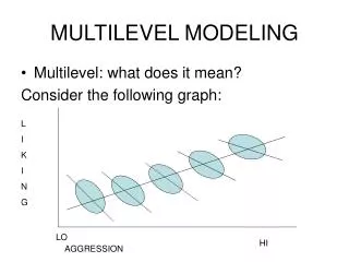
Individuals Undivided Unit of Analysis = Individuals
Individuals Nested Within Groups Unit of Analysis = Individuals + Classes
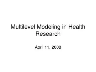
… and Further Nested Unit of Analysis = Individuals + Classes + Schools
Examples of Multilevel Data Structures • Neighborhoods are nested within communities • Families are nested within neighborhoods • Children are nested within families
Examples of Multilevel Data Structures • Schools are nested within districts • Classes are nested within schools • Students are nested within classes
Multilevel Data Structures Level 4 District (l) Level 3 School (k) Level 2 Class (j) Level 1 Student (i)
2nd Type of Nesting • Repeated Measures Nested Within Individuals Focus = Change or Growth
Nested Data • Data nested within a group tend to be more alike than data from individuals selected at random. • Nature of group dynamics will tend to exert an effect on individuals.
Nested Data • Intraclass correlation (ICC) provides a measure of the clustering and dependence of the data 0 (very independent) to 1.0 (very dependent) Details discussed later
Multilevel Modeling Seems New But…. Extension of General Linear Modeling Simple Linear Regression Multiple Linear Regression ANOVA ANCOVA Repeated Measures ANOVA
Why Multilevel Modelingvs. Traditional Approaches? Traditional Approaches – 1-Level • Individual level analysis (ignore group) • Group level analysis (aggregate data and ignore individuals)
Problems withTraditional Approaches • Individual level analysis (ignore group) Violation of independence of data assumption leading to misestimated standard errors (standard errors are smaller than they should be).
Problems withTraditional Approaches • Group level analysis (aggregate data and ignore individuals) Aggregation bias = the meaning of a variable at Level-1 (e.g., individual level SES) may not be the same as the meaning at Level-2 (e.g., school level SES)
Example: Paired t-test: the average change in DBP is significantly different from zero (p = 0.000951) Unpaired t-test: the average change in DBP is significantly different from zero (p = 0.036)
Multilevel Approach • 2 or more levels can be considered simultaneously • Can analyze within- and between-group variability
How Many Levels Are Usually Examined? 2 or 3 levels very common 15 students x 10 classes x 10 schools = 1,500
Types of Outcomes • Continuous Scale (Achievement, Attitudes) • Binary (pass/fail) • Categorical with 3 + categories
Effect for estimation of a mean • if the sample is a two-stage sample using random sampling with replacement at either stage or if the sampling fractions are so low that the difference between sampling with and sampling without replacement is negligible.
Effect for estimation of a mean • Since considerations for the choice of a design always are of an approximate nature, only those designs are considered here where each level-two unit contains the same number of level-one units. • Level-two units will sometimes be referred to as clusters. The number of level-two units is denoted N • The number of level-one units within each level-two unit is denoted n • These numbers are called the level-two sample size and the cluster size, respectively • The total sample size is Nn. • If in reality the number of level-one units fluctuates between level-two units, it will almost always be a reasonable approximation to use for n the average number of sampled level-one units per level-two unit.
Effect for estimation of a mean • Suppose that the mean is to be estimated of some variable Y in a population which has a two-level structure. As an example, Y could be the duration of hospital stay after a certain operation under the condition that there are no complications or additional health problems. Random Intercept
Effect for estimation of a mean This increase in complexity permeates to regression, etc This is a relatively simple model, more complex models lead to more complex calculations that require the calculation of large covariance matrices
Easier Case The effect of each level-2 unit is a constant (fixed), not a random variable Another alternative to this operation is to add a dummy variable for each individual
Software to do Multilevel Modeling SAS Users PROC MIXED Extension of General Linear Modeling Simple Linear Regression Multiple Linear Regression ANOVA ANCOVA Repeated Measures ANOVA PROC REG PROC GLM PROC ANOVA
Example: Family and Gender • The response variable Height measures the heights (in inches) of 18 individuals. • The individuals are classified according to Family and Gender data heights; input Family Gender$ Height @@; datalines; 1 F 67 1 F 66 1 F 64 1 M 71 1 M 72 2 F 63 2 F 63 2 F 67 2 M 69 2 M 68 2 M 70 3 F 63 3 M 64 4 F 67 4 F 66 4 M 67 4 M 67 4 M 69 ; run; Different than “Effects…” because now we have more cluster levels, but no random intercepts
Example: Family and Gender • The PROC MIXED statement invokes the procedure. The CLASS statement instructs PROC MIXED to consider both Family and Gender as classification variables. • Dummy (indicator) variables are, as a result, created corresponding to all of the distinct levels of Family and Gender. • For these data, Family has four levels and Gender has two levels. proc mixed data=heights; class Family Gender; model Height = Gender Family Family*Gender/s; run; s : requests that a solution for the fixed-effects parameters be produced along with their approximate standard errors
Family and Gender • Run program simple-proc_mixed2.sas What happens when you try to use the statement CLASS in a PROC REG? Ordinary Linear Regression coefficients are just one set of them, while for HLM coefficients are estimated for each group unit (i.e., school)
Dorsal shells in lizards Two-sample t-test: the small observed difference is not significant (p = 0.1024).
Mother effect • We have 102 lizards from 29 mothers • Mother effects might be present • Hence a comparison between male and female animals should be based on within-mother comparisons.
Mother effect # of dorsal shells Mother
First Choice Β can be interpreted as the average difference between males and females for each mother Test for a ‘sex’ effect, correcting for ‘mother’ effects, More complex example than “Effect…” because now we have a variable xij for each observation
SAS program Notice that in the previous example “Family and Gender” , gender was a used to define level(cluster) here is just a variable. In previous example it was assumed that individual of the same gender were “clustered”/correlated? Now it is just an input variable proc mixed data = lizard; class mothc; model dors = sex mothc; run; Source F Value Pr > F SEX 7.19 0.0091 MOTHC 3.95 <.0001 Highly significant mother effect. Significant gender effect. Many degrees of freedom are spent to the estimation of the mother effect, which is not even of interest
Later in this semester… • Note the different nature of the two factors: • SEX: defines 2 groups of interest • MOTHER: defines 29 groups not of real interest. A new sample would imply other mothers. • In practice, one therefore considers the factor ‘mother’ as a random factor. • The factor ‘sex’ is a fixed effect. • Thus the model is a mixed model. • In general, models can contain multiple fixed and/or random factors. Fixed Effects Model Random Effects Model As in the slides of “Effect…”
Later in this semester… • Note the different nature of the two factors: • SEX: defines 2 groups of interest • MOTHER: defines 29 groups not of real interest. A new sample would imply other mothers. • In practice, one therefore considers the factor ‘mother’ as a random factor. • The factor ‘sex’ is a fixed effect. • Thus the model is a mixed model. • In general, models can contain multiple fixed and/or random factors. proc mixed data = lizard; class mothc; model dors = sex / solution; random mothc; run;
More terminology • Fixed coefficient • A regression coefficient that does not vary across individuals • Random coefficient • A regression coefficient that does vary across individuals
Is a variable random or fixed effect? • LaMotte 1983, pp. 138–139 • Treatment levels used are the only ones about which inferences are sought => fixed Effect • Inferences are sought about a broader collection of treatment effects than those used in the experiment, or if the treatment levels are not selected purposefully => Random Effect
More terminology • Balanced design • Equal number of observations per unit • Unbalanced design • Unequal number of observation per unit • Unconditional model • Simplest level 2 model; no predictors of the level 1 parameters (e.g., intercept and slope) • Conditional model • Level 2 model contains predictors of level 1 parameters
Weighted Data Problem: Pct. of Voting Population Pct. of People who have a phone Minority Voters Minority Voters White Voters White Voters Solution: Give more “weight” to the minority people with telephone
Weighted Data Not limited to 2 categories Pct. of Voting Population Pct. of People who have a phone Minority/Dem. Minority/Dem. Minority/Rep. Minority/Rep. White /Dem White /Dem White /Rep White /Rep How many categories? As many as there are significant
Proportion Suppose minority voters are 1/3 of the voting population but only 1/6 of the people with phone A sampling weight for a given data point is the number of receipts in the target population which that sample point represents. Needless to say that in reality this is a much more complex issue
Which weight we need to use? • Oversimplified example (don’t take seriously) Pct. of Voting Population in 2008 Pct. of People who have a phone Minority Voters O Minority Voters White Voters Pct. of Voting Population in 2010 White Voters Minority Voters M White Voters
Proportion Suppose minority voters are 1/3 of the voting population but only 1/6 of the people with phone • 100 minority + 500 white answer the phone survey • 75 Minority will vote for candidate X • 250 White will votes for candidate X • Non-Weighted Conclusion: 325/600 =54.16% of the voters will vote for candidate X • Weighted Conclusion: • 75 minority = 75% of minority with phone=>(.75)*(1/6)=12.5% of people with phone * 2 weight= 25% pct of voting population • 250 white = 50% of white people with phone =>(.5)*(5/6)= 41.66% of people with phone * .8 weight =>33.33% • 25% +33.33%=58.33%
SAS Weighted Mean proc means data=sashelp.class; var height; run; proc means data=sashelp.class; weight weight; var height; run;
Weighted PROC MIXED proc mixed data=sashelp.class covtest; class Sex; model height=Sex Age/solution; weight weight; run; proc mixed data=sashelp.class covtest; class Sex; model height=Sex Age/solution; weight weight; run; Notice the difference (kind of small) in let’s say the coefficients of the model (Solution for Fixed Effects/Estimates)
Farms Example • It's stratified by regions within Iowa and Nebraska. • Regress on farm area, with separate intercept and slope for each state
References • LaMotte, L. R. (1983). Fixed-, random-, and mixed-effects models. In Encyclopedia of Statistical Sciences, S. Kotz, N. L. Johnson, and C. B. Read