Introduction to Multilevel Modeling

1. Introduction to Multilevel Modeling Stephen R. Porter Associate Professor Dept. of Educational Leadership and Policy Studies Iowa State University Lagomarcino Hall Ames, IA 50011 Email: srporter@iastate.edu

2. Goals of the workshop • Understand why multilevel modeling is important and understand basic 2-level models. • Become informed consumer of multilevel research. • Know how to estimate some simple models using the software package HLM. • Have a thorough grounding in the basics so you can learn more complicated multi-level techniques (3-level, SEM, etc.) on your own.

3. Schedule • 1st day • Review and discuss multilevel terminology and theory • Begin reviewing choices in model building • 2nd day • Estimate simple 2-level models using student version of HLM • Discuss in detail model building.

4. Introduction

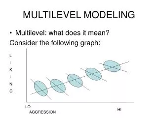
5. Why multilevel modeling? • Nested data are very common in higher education. • Analysis of nested data poses unit of analysis problem – should we analyze the individual or the group? Unfortunately, we often can’t choose one over the other. • Traditional linear models offer a simple view of a complex world – generally assume same effects across groups. • If effects do differ across groups, we can explain these differences with multilevel modeling.

6. Unit of analysis problem: individual, group or both? • Example: studying what affects student retention (1000 students per college) in a group of colleges (n=50). Total dataset N=50,000. • We can assign college-level variables to each individual, but … • We end up estimating the standard errors for college-level variables using N=50,000. • Yet we only have 50 different college observations, so N really equals 50.

7. Unit of analysis problem: individual, group or both? • Alternatively, we can average student data for each college so that we have 1 observation per college (N=50). • Now we have reduced variance on our student-level variables. • We also have variables which measure both individual student characteristics (SAT score=aptitude/preparation) and college environment (average SAT score=selectivity).

8. What are nested data? • Simply put, sub-units are grouped (or “nested”) within larger units. • Often the data are observations of individuals nested within groups. • Key: individuals within groups are more similar to one another than to individuals in other groups. • We can empirically verify this. • Sometimes data are multiple observations nested within an individual.

9. Students/faculty nested withindepartments/disciplines Note that this could be one institution, or individuals from several different institutions. Examples: student satisfaction, gains in skills; faculty salaries, research productivity.

10. Students/faculty nested withininstitutions Examples: student satisfaction, retention

11. Time periods nested within students Example: grade-point average

12. Terms and theory

13. Terminology: HLM • HLM stands for hierarchical linear models. • It is both a statistical technique and a software package. • People also use the term multilevel models. • Economists often refer to these models as random-coefficient regression models

14. Terminology: levels • Level-1 variables: • These are the variables that are nested within groups. • Typically these are individual-level variables. • Level-2 variables • Typically these are unit-level variables. • Note that growth models have time periods at level-1, and individuals at level-2.

15. Terminology: variance Numbers represent people, each number is a person’s question response on a 5-point Likert scale; 6 groups Variance between groups only: 1111 2222 5555 4444 2222 3333 Variance within groups only: 1235 1235 1235 1235 1235 1235 Variance both between and within groups: 1112 2233 2333 3344 3444 4455

16. Terminology: random and fixed • Fixed effects are variable coefficients that are constant across groups, they do not vary. • Typical OLS coefficients. • Random effects are coefficients that can vary across groups. • This means the coefficient can take a different value for each group. E.g., if we allow an intercept for each group, then the intercept is said to be random. • It is random because we assume it is stochastic. • Yet we can also explain some of this variance with other variables.

17. One way to think about multilevel models: “slopes-as-outcomes” • Suppose we estimate 1 regression equation for each group, e.g., for the 1,000 students in school A, the 1,000 students in school B, etc. The result is 50 regression equations. • We then take the slope coefficients for each school, as well as information about each school such as private/public status, and make a new dataset. • We run a regression model on these 50 observations using the slope coefficients (or intercepts) as the dependent variable and public/private status as the independent variable. • The result is a single set of coefficients for the school dataset.

18. Now for some algebra! • You must learn some of the basic mathematical notation used in multilevel modeling. • As we will see, the program HLM uses this notation to express the models that you estimate. • Understanding these basic symbols and expressions will allow you to tackle more complex analyses, and understand other researchers’ more complex analyses.

19. A level-1 model: multiple students in one school (familiar OLS equation) • Student i is viewed as having average achievement in the school, plus a positive deviation due to SES, plus a positive or negative deviation due to the unique circumstances of the student.

20. A level-1 model: multiple students in multiple schools • Now we’re estimating the equation from before for each school. Each school can have a different average achievement (or intercept), and a different impact of SES on achievement (or slope).

21. Need to make some additional assumptions about the coefficients, because they vary • Student-level errors are normally distributed. • Gamma’s: we expect the average achievement for school j to equal the average school mean for all j schools, and the slope of SES for school j to equal the average of the slopes for all j schools. • Tau’s: these are the variances of the intercepts and slopes, and the covariance between them.

22. Level-2 model: explaining the Level-1 coefficients • Since our intercepts and slopes vary by school, we can now model why they vary. • Suppose we hypothesize that levels of achievement and impact of SES are related to whether a school is public or Catholic. • We need equations for the intercept and slope to describe our hypothesis:

23. Level-2 model: continued

24. So math achievement of an individual student in school j is explained by … mean achievement in public schools, plus impact of a school being Catholic on mean achievement (if j is Catholic) the effect of SES on achievement, plus the impact of a school being Catholic on how SES affects achievement (again, if j is Catholic) student- and school-specific error terms

25. Summary Level-1 Explain dependent variable Level-2 Explain slopes Level-2 Explain intercepts

26. Some practical aspects of multilevel modeling

27. Questions to answer • Canyou use multilevel techniques to study your dependent variable? • Shouldyou use multilevel techniques to study your dependent variable? • How will you center your level-1 and level-2 predictors? • Which of the level-1 coefficients will be explained at level-2? I.e., are they fixed or random? • How does my model perform?

28. Can I use HLM? • HLM requires a large amount of data. • Minimum: • number of groups: 30, but most recommend 50+ • number of individuals within groups: 5-10, but can have low as 1. • average group size: 10, obviously more is better.

29. Should I be using HLM? • How much of the variance in your dependent variable is explained by group membership? • Intraclass correlation coefficient (ICC) = var between groups (var between groups+var within groups)

30. Centering variables • Whether and how you center is a very important decision: interpretation of results depends on your choice. • Important because the intercept at level-1 is also a dependent variable. • Centering • Refers to subtracting a mean from your independent variables. • The transformed value for an individual measures how much they deviate (+/-) from the mean.

31. Centering variables • Suppose we center verbal SAT scores around a student mean of 500. • How would we interpret a regression coefficient if all variables were similarly transformed?

32. Centering variables • Why would we want to center? • Variable may lack a natural zero point, such as SAT score. • Stability of estimates at level-1 affected by location of variables. • Location at level-2 is less important.

33. Centering variables • Generally two types of centering. For a specific variable: • Grand mean centering – subtract the mean for the entire sample from each observation in the sample. • Group mean centering – subtract the mean for each group from each member of the group. • To fully understand the implications of centering, see the discussion in Bryk and Raudenbush (2002) pp. 134-149.

34. Fixed or random? • It would be nice to have everything random; that is, a different set of coefficients for each group. • But due to HLM demands on data, usually only the intercept and a few variables can be random. • Important: if you randomize gender and you have a group without females, that group will be dropped. • Generally you should run parallel models for intercept and slopes, as in our theory example.

35. Model statistics • Goodness of fit: • Proportion of variance explained at level-1 • Variance explained at level-2

36. Some thoughts about building your models • Before using HLM, run OLS regressions for sample and for each group. • Building the null model: • This is should be your first step. • Calculate the ICC • Building the level-1 models: • Should be theory driven • Step-up approach • Be cautious about what you leave as random – it’s often difficult to leave more than the intercept and one variable as random

37. Some thoughts about building your models • Building the level-2 models • Rule of thumb: 10 observations/variable • Parallel models • Many scholars drop insignificant variables at both levels. (I disagree with this.)