Download
1 / 27
270 likes | 423 Views
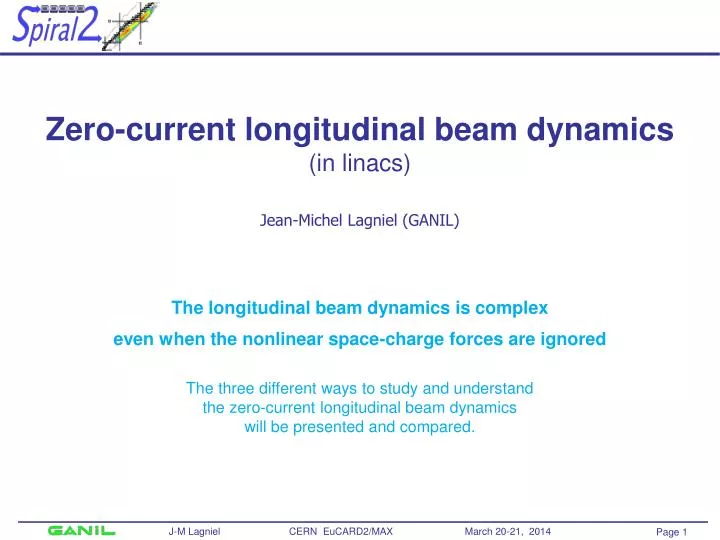
Zero-current longitudinal beam dynamics (in linacs) Jean-Michel Lagniel (GANIL) The longitudinal beam dynamics is complex even when the nonlinear space-charge forces are ignored The three different ways to study and understand the zero-current longitudinal beam dynamics

E N D
Zero-current longitudinal beam dynamics (in linacs) Jean-Michel Lagniel (GANIL) The longitudinal beam dynamics is complex even when the nonlinear space-charge forces are ignored The three different ways to study and understandthe zero-current longitudinal beam dynamics will be presented and compared. J-M Lagniel CERN EuCARD2/MAX March 20-21, 2014
The 3 ways to study the longitudinal beam dynamics Synchronous particle and oscillations around the synchronous particle J-M Lagniel CERN EuCARD2/MAX March 20-21, 2014
Program I- EoM integration in field maps Mappings II- Mappings 2nd order differential EoM III- Longitudinal beam dynamics without damping Smooth approximation vs Mapping vs Integration in field map IV- Longitudinal beam dynamics with damping Smooth approximation vs Mapping vs Integration in field map V- Concluding remark J-M Lagniel CERN EuCARD2/MAX March 20-21, 2014
I- From EoM integration in field maps to mappings Numerical integration (dz) of the EoM in field maps (, W) phase-space J-M Lagniel CERN EuCARD2/MAX March 20-21, 2014
I- From EoM integration in field maps to mappings Mappingi+1 = i + Wi+1 = Wi + W => Integration over one accelerating cell - cavity (z = 0) Ez mean value (Panofsky 1951)The Transit-Time-Factor contains all the information on the field map and speed + radial evolution over the accelerating cell / cavity Without approximation More complicated than the original ! only useful with approximations J-M Lagniel CERN EuCARD2/MAX March 20-21, 2014
I- From EoM integration in field maps to mappings Odd function of z Ez(r,z) = even function + constant speedand radius over the cell Constant speed and radius over the cell The TTF of each particle is a function of the particle mean radius and velocities (input values in practice) but not function of the particle radius and speed evolution over the cell J-M Lagniel CERN EuCARD2/MAX March 20-21, 2014
I- From EoM integration in field maps to mappings Allows to find analytical expressions of the TTF for particular field distributions J-M Lagniel CERN EuCARD2/MAX March 20-21, 2014
I- From EoM integration in field maps to mappings Using an approximated formula to evaluate the particle TTF we have found a practical way to build a mapping NO ! This mapping is not (by far) symplectic (area preserving) when the TTF is calculated taking into account the particle mean speed and radius A phase correction must be added to obtain a symplectic mapping (1st order) Pierre Lapostolle et al 1965 – 1975 (B.C. age). J-M Lagniel CERN EuCARD2/MAX March 20-21, 2014
I- From EoM integration in field maps to mappings The only way to produce a simple symplectic mapping is to consider the synchronous particle TTF for every particle TTF analytical expression => neglect the evolution of the velocity in the cell Simple symplectic mapping => neglect the effect of the particle velocity spread on the TTF (Phase and energy evolution with respect to the synchronous particle) J-M Lagniel CERN EuCARD2/MAX March 20-21, 2014
II- From mappings to 2nd order differential EoM Smooth approximation considering the mapping without phase correction Large amplitude oscillations Long term behavior Low amplitude oscillations Error J-M Lagniel CERN EuCARD2/MAX March 20-21, 2014
III- Longitudinal beam dynamics without damping Smooth approximation(2nd order Differential EoM obtained using the smooth approximation) Particle trajectories – separatrix vs synchronous phase s = -90° s = -30° J-M Lagniel CERN EuCARD2/MAX March 20-21, 2014
III- Longitudinal beam dynamics without damping Smooth approximation Choice of s -20° -15° Long. Acceptance / 2 €€€ The temptation is high to increase the synchronous phase €€€ High-power LINAC designers (and managers) must bringas much attention to the longitudinal beam size / longitudinal aperture ratioas they bring to the radial beam size / radial aperture ratio J-M Lagniel CERN EuCARD2/MAX March 20-21, 2014
III- Longitudinal beam dynamics without damping Smooth approximationvs Mapping s = -90° J-M Lagniel CERN EuCARD2/MAX March 20-21, 2014
III- Longitudinal beam dynamics without damping Mapping s = -90° 0l* > 50° More and more resonances => resonance overlaps=> larger choatic area 82°, 86°, 90° / lattice => real phase advance value higher than the one given by the smooth approximation J-M Lagniel CERN EuCARD2/MAX March 20-21, 2014
III- Longitudinal beam dynamics without damping As 0l* increases the phase-space portraits plotted using the mapping show more and more resonances more and more resonance overlaps larger and larger choatic areas longitudinal acceptance reduction [ Fateev & Ostroumov NIM 1984 ] [ Bertrand, EPAC04 ] Is it true or is it a spurious effect of the mapping ? ( periodic error = excitation of the resonances ? ) ... If yes, why ? Check making a direct integration of the EoM J-M Lagniel CERN EuCARD2/MAX March 20-21, 2014
III- Longitudinal beam dynamics without damping Longitudinal toy Direct integration of the EoMs = -90° h frf TTF Field map = First-harmonic-model 0l* Epic J-M Lagniel CERN EuCARD2/MAX March 20-21, 2014
III- Longitudinal beam dynamics without damping Phase-space portraits plotted using the Longitudinal Toy 0l* = 80° Lc = L h = 1 Ez(z) = pure sinusoid (first-harmonic) 1/4 resonance not excited !!!! 0l* = 90° 0l* = 95° J-M Lagniel CERN EuCARD2/MAX March 20-21, 2014
III- Longitudinal beam dynamics without damping Phase-space portraits plotted using the Longitudinal Toy 0l* = 50° Lc = L/4 h = 4 Ez(z) with harmonics > 1 The resonances are excited Mapping 0l* = 90° 0l* = 70° J-M Lagniel CERN EuCARD2/MAX March 20-21, 2014
III- Longitudinal beam dynamics without damping summary EoM @ smooth approximation Ez(z) = Constant => Resonances not excited ... but essential to understand the longitudinal beam dynamics Physics Mapping Ez(z) = Dirac comb (period L) => FT[Ez(z)] = Dirac comb (1/L) All resonances excited EoM using field maps Ez(z) = Field map => FT[Ez(z)] = some harmonics (1/L) Some resonances excited (need more work !) The longitudinal acceptance can be significantly reduced at high 0l* J-M Lagniel CERN EuCARD2/MAX March 20-21, 2014
IV- Longitudinal beam dynamics with damping Smooth approximation (, ’) plane Attractor = (0, 0) s = -30° Basin of attraction Acceptances + separatrix K = 0 J-M Lagniel CERN EuCARD2/MAX March 20-21, 2014
IV- Longitudinal beam dynamics with damping Mapping (, ’) plane Attractors = (0, 0) and the 1/4 resonance islands 0l* = 82° J-M Lagniel CERN EuCARD2/MAX March 20-21, 2014
IV- Longitudinal beam dynamics with damping Mapping Basin of attraction (, ’) plane K = 0.02 K = 0.10 0l* = 60° K = 0.01 K = 0.10 0l* = 70° Attractors : (0, 0) (1/6 resonance) J-M Lagniel CERN EuCARD2/MAX March 20-21, 2014
IV- Longitudinal beam dynamics with damping Mapping (fractal) Basin of attraction (, d/ds) plane K = 0.05 K = 0.01 0l* = 82° Attractors(0, 0)(1/4 resonance) K = 0.20 K = 0.10 J-M Lagniel CERN EuCARD2/MAX March 20-21, 2014
IV- Longitudinal beam dynamics with damping ESS linac (2012) K = 0.36 … 0.10 … 0.04 DTL 0.015 … 0.005 highenergy J-M Lagniel CERN EuCARD2/MAX March 20-21, 2014
IV- Longitudinal beam dynamics with damping SPIRAL 2 superconducting linac K = 0.05 … 0.08 … 0.12 … 0.19 … 0.16 … 0.08 … 0.05 J-M Lagniel CERN EuCARD2/MAX March 20-21, 2014
IV- Longitudinal beam dynamics with damping Summary The stable fix points of the resonance islandsact as main attractors at low damping rates The damping can annihilate the effect of the resonances • k should be considered as an important parameter • to analyze a linac design and understand its longitudinal beam dynamics J-M Lagniel CERN EuCARD2/MAX March 20-21, 2014
Concluding remark Hope you are now convinced that thezero-current longitudinal beam dynamics is complex ! !!! At least more complex than what is taught inclassical Accelerator Books and Accelerator Schools !!! J-M Lagniel CERN EuCARD2/MAX March 20-21, 2014