Download
1 / 1
10 likes | 178 Views
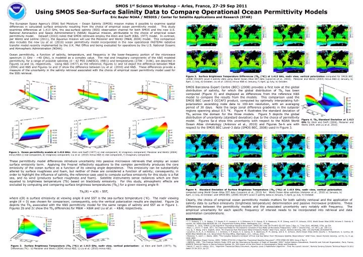
SMOS 1 st Science Workshop – Arles, France, 27-29 Sep 2011 Using SMOS Sea-Surface Salinity Data to Compare Operational Ocean Permittivity Models Eric Bayler NOAA / NESDIS / Center for Satellite Applications and Research (STAR).

E N D
SMOS 1st Science Workshop – Arles, France, 27-29 Sep 2011 Using SMOS Sea-Surface Salinity Data to Compare Operational Ocean Permittivity Models Eric Bayler NOAA / NESDIS / Center for Satellite Applications and Research (STAR) The European Space Agency’s (ESA) Soil Moisture – Ocean Salinity (SMOS) mission makes it possible to examine spatial differences in calculated surface emissivity resulting from the choice of empirical ocean permittivity model. This study examines differences at 1.413 GHz, the sea-surface salinity (SSS) observation channel for both SMOS and the new U.S. National Aeronautics and Space Administration’s (NASA) Aquarius mission, attributable to the choice of empirical ocean permittivity model. Delwart (2010) notes that SMOS retrievals employ the Klein and Swift (K&S, 1977) model. In contrast, per Wentz and LeVine (2011), the Aquarius mission will use the Meissner and Wentz (M&W, 2004) model. This comparison also includes the new Liu et al. (2010) ocean permittivity model incorporated in the new operational FASTEM4 radiative transfer model recently implemented by the U.K. Met Office and being evaluated for operations by the U.S. National Oceanic and Atmospheric Administration (NOAA). Ocean permittivity, a function of salinity, temperature, and frequency in the lower-frequency portion of the microwave spectrum (1 GHz - ~40 GHz), is modeled as a complex value. The real and imaginary components of the K&S modeled permittivity, for a range of possible salinities (0 - 42 PSS (UNESCO, 1981)) and temperatures (270K - 310K), are depicted in Figures 1a and 1b, respectively. Using K&S (1977) as the reference, Figures 1c and 1d depict the difference between M&W (2004) and K&S and Figures 1e and 1f show the difference between Liu et al. (2010) and K&S. These differences provide a measure of the uncertainty in the salinity retrieval associated with the choice of empirical ocean permittivity model used for the SSS retrieval. a b c d a b c Figure 2. Surface Brightness Temperature (Tb0 (°K)) at 1.413 GHz, nadir view, vertical polarization: a) Klein and Swift (1977); Tb0 Differences (°K): b) Meissner and Wentz (2004) minus K&S, c) Liu et al. (2010) minus K&S. e f g h Figure 3. Surface Brightness Temperature Differences (Tb0 (°K)) at 1.413 GHz, nadir view, vertical polarization computed for SMOS BEC (2008) OCCAF3 Level-3 salinity data using World Ocean Atlas SST data (Locarnini et al., 2010): Meissner and Wentz (2004) minus K&S a) January, b) April, c) July, d) October; Liu et al. (2010) minus K&S e) January, f) April, g) July, h) October. a c e SMOS Barcelona Expert Centre (BEC) (2008) provides a first look at the global distribution of salinity, for which the global distribution of Tb0 has been computed (Figure 3) and displayed as differences from the reference K&S model to compare the results from the models. This comparison used the SMOS BEC Level-3 OCCAF3 product, computed by optimally interpolating full-polarization ascending node data to 100-km resolution, with an averaging period of 30 days. Note the large zonal difference gradients in the subpolar regions spanning about 0.5 °K. Figure 4 illustrates the standard deviation of Tb0 across the domain for the three models. Figure 5 depicts the global distribution of uncertainty (standard deviation) due to the choice of permittivity model. Figures 5a-d show this uncertainty with respect to the NOAA World Ocean Atlas climatology (Antonov et al., 2010) and Figures 5e-h are with respect to the SMOS BEC Level-3 data (SMOS BEC, 2008) used in Figure 3. b d f Figure 1. Ocean permittivity models at 1.413 GHz: Klein and Swift (1977) a) real component, b) imaginary component; Meissner and Wentz (2004) minus K&S c) real component, d) imaginary component; Liu et al. (2010) minus K&S e) real component, f) imaginary component. These permittivity model differences introduce uncertainty into passive microwave retrievals that employ an ocean surface emissivity term. Applying the Fresnel reflectivity equations to the complex permittivity produces the core emissivity of the ocean surface as a function of its viewing angle dependence. This emissivity can be substantially altered by surface roughness and foam, but neither of these are considered a function of salinity; consequently, in order to highlight the influence of salinity, the reference case used to compute surface emissivity for this study is a flat sea, and no wind (produces surface roughness and foam). Satellite instruments sense radiances which are then equated to brightness temperature (Tb) based on blackbody emissivity. For this study, atmospheric effects are excluded by computing and comparing surface brightness temperatures (Tb0) for a given viewing angle θ: Tb0(θ) = ε(θ) SST, where ε(θ) is surface emissivity at viewing angle θ and SST is the sea-surface temperature (K). The nadir viewing angle (θ = 0) was chosen for comparison; consequently, only the vertical polarization results are depicted. Figure 2a depicts the Tb0 associated with the K&S permittivity model for the same ranges of salinity and SST as in Figure 1. Figures 2b and 2c show the Tb0 differences for M&W – K&W and Liu et al. – K&W, respectively. Figure 4. Tb0 Standard Deviation at 1.413 GHz for Klein and Swift (2004), Meissner and Wentz 2004, and Liu et al. 2010) a b c d Clearly, the choice of empirical ocean permittivity models matters for both salinity retrieval and the application of salinity data to surface emissivity (brightness temperature) determination and passive microwave problems. These differences between the permittivity models and the associated uncertainty vary notably with frequency. The empirical uncertainty for each specific frequency of interest needs to be incorporated into retrieval and data assimilation considerations. • REFERENCES: • J. I., Antonov, J. I., D. Seidov, T. P. Boyer, R. A. Locarnini, A. V. Mishonov, H. E. Garcia, O. K. Baranova, M. M. Zweng, and D. R. Johnson, 2010, World Ocean Atlas 2009, Volume 2: Salinity. S. Levitus, Ed. NOAA Atlas NESDIS 69, U.S. Government Printing Office, Washington, D.C., 184 pp. • Delwart, S., 2010, “SMOS L2 OS Algorithm Theoretical Baseline Document”, SMOS Doc code SO-TN-ARG-GS-007 Issue 3 Rev: 6, 7 Dec 2010, ARGANS / ESA, pp 234. • Klein, L., and C. T. Swift, 1977, “An Improved Model for the Dielectric Constant of Sea Water at Microwave Frequencies,” IEEE J. Oceanic Eng., vol. OE-2, pp. 104-111. • Liu, Q., F. Weng, and S. English, 2010, “An Improved Fast Microwave Water Emissivity Model,” IEEE Trans. Geosci. Remote Sensing, DOI: 101109/TGRS.20102064779. • Locarnini, R. A., A. V. Mishonov, J. I. Antonov, T. P. Boyer, H. E. Garcia, O. K. Baranova, M. M. Zweng, and D. R. Johnson, World Ocean Atlas 2009, Volume 1: Temperature. S. Levitus, Ed. NOAA Atlas NESDIS 68, U.S. Government Printing Office, Washington, D.C., 184 pp, 2010. • Meissner, T., and F. J. Wentz, 2004, “The Complex Dielectric Constant of Pure and Sea Water From Microwave Satellite Observations,” IEEE Trans. Geosci Remote Sensing, vol 42, no. 9, pp. 1836-1849. • SMOS Barcelona Expert Centre, 2008, “SMOS CP34 OS L3 Algorithm Theoretical Baseline Document”, CP34-ATBD-OS-0001 Issue 2 Rev 3. • UNESCO, 1981, “The Practical Salinity Scale 1978 and the International Equation of State of Seawater 1980,” United Nations Educational, Scientific and Cultural Organization, Paris, France, UNESCO Technical Papers in Marine Science Number 36, 10th report of the Joint Panel on Oceanographic Tables and Standards. • Wentz, F., and D. LeVine, 2011, “Algorithm Theoretical Basis Document, Aquarius Level-2 Radiometer Algorithm: Final Pre-Launch Version”, Remote Sensing Sytems Technical Report 011811 dated 18 Jan 2011, pp 23. e f g h Figure 5. Standard Deviation of Surface Brightness Temperature (Tb0 (°K)) at 1.413 GHz, nadir view, vertical polarization computed using World Ocean Atlas SST data (Locarnini et al., 2010) for: World Ocean Atlas salinities (Antonov et al., 2010) a) January, b) April, c) July, d) October; and SMOS BEC (2008) OCCAF3 Level-3 salinity data e) January, f) April, g) July, h) October.