Sociology 601 Class 13: October 13, 2009

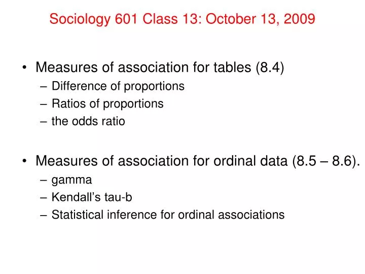
Sociology 601 Class 13: October 13, 2009 • Measures of association for tables (8.4) • Difference of proportions • Ratios of proportions • the odds ratio • Measures of association for ordinal data (8.5 – 8.6). • gamma • Kendall’s tau-b • Statistical inference for ordinal associations

8.4: Measures of Association: Difference of Proportions The difference of proportions is the proportion scoring “yes” in one category of variable X, minus the proportion scoring “yes” in another category of variable X. Formal definition: For two variables X and Y, with 1,2 as possible values for X and 1,2 as possible values for Y: d. p. = P ((Y = 1) | (X = 1)) - P ((Y = 1) | (X = 2)) alternately, d. p. = x=1|y=1 - x=1|y=2

Example for difference of proportions difference of proportions = yes|40+ - yes|<40 = .35 - .49 = -.14 The sample percent of older people (40+) who support abortion is 14 percentage points lower than the percent of younger people (under 40) who support abortion

Difference of proportions: the problem A difference of proportions calculated at about .5 does not seem as important as the same difference calculated near 0.0 or 1.0. Fictitious example: women as a proportion of all veterinary school students. 1960, p=.02 1965, p=.06, difference = .04 1990, p =.51 1995, p=.55 difference = .04 2020, p =.94 2025, p=.98 difference = .04 which 5-year span reflects the largest underlying social change?

Measures of association: Odds and odds ratios • Odds = proportion of one response • proportion of other response • Examples: what are the odds that a veterinary student would be a woman in 1990? 1995? 1960? 1965? 2020? 2025? • 2025, p=.98, odds= 49.0 (or 49 : 1) • 2020, p =.94, odds= 15.7 (or 15.7 : 1) • 1995, p=.55 odds= 1.22 (or 1.22 : 1) • 1990, p =.51 odds= 1.04 (or 1.04 : 1) • 1965, p=.06, odds= 0.0638 (or 1 : 15.7) • 1960, p=.02, odds= 0.0204 (or 1 : 49)

Problems with Odds and odds ratios • Not as intuitively obvious as difference in proportions • The odds tend to take extreme values when the proportion under consideration is near 1 or zero. • Odds are not symmetric around 50-50 = 1.0 • So, we often take log odds: • log (4:1) = - log(1:4) • But this is even less intuitive.

Odds ratios • 2025, odds= 49.0; 2020, odds= 15.7; ratio= 3.12 • 1995, odds= 1.22; 1990, odds= 1.04; ratio= 1.17 • 1965, odds= 0.0638; 1960, odds= 0.0204; ratio= 3.12

8.5. Stepping up to ordinal and interval data • The chi-squared test is an extremely simple test of relationships between categories. • In chi-squared tests, we ask “Does the distribution of one variable depend on the categories for the other variable?” • This sort of question requires only nominal-scaled data • We are usually interested in more informative tests of relationships between categories. • In such tests, we ask “As we increase the level of one variable, how do we change the level of another?” • “The more of X, the more of Y”

A weakness of a chi-squared test. • The problem: Chi-Squared tests are for nominal associations. If we use a chi-squared test when there is an ordinal association, we waste some information. Chi-Squared tests cannot distinguish the following patterns:

Alternative for ordinal data A solution: find concordant and discordant patterns. • Identify every possible pair of observations. The number of possible pairs far exceeds the number of observations. • A pair of observations is concordant if the subject who is higher on one variable is also higher on the other variable. • A pair of observations is discordant if the subject who is higher on one variable is lower on the other variable. • Many pairs of observations are neither concordant nor discordant (i.e., ties). We ignore those pairs.

Finding concordant and discordant patterns. • For all but the smallest samples, the number of concordant and discordant patterns can be very difficult to count, so we usually leave that exercise to a computer program. • It is, however, important to understand what the computer is doing. For that reason, we will try an example. Concordant pairs: Discordant pairs:

Counting concordant pairs (no like, low wages) x (maybe like, med wages) = 10 x 4 = 40 (no, low) x (maybe, high) = 10 x 7 = 70 (no, low) x (yes, med) = 10 x 5 = 50 (no, low) x (yes, high) = 10 x 2 = 20 (maybe, low) x (yes, med) = 1 x 5 = 5 (maybe, low) x (yes, high) = 1 x 2 = 2 (no, med) x (maybe, high) = 3 x 7 = 21 (no, med) x (yes, high) = 3 x 2 = 6 (maybe, med) x (yes, high) = 4 x 2 = 8 Total concordant pairs = 222

Counting discordant pairs (no like, med wages) x (maybe like, low wages) = 3 x 1 = 3 (no, med) x (yes, low) = 3 x 1 = 3 (no, high) x (maybe, med) = 3 x 4 = 12 (no, high) x (yes, med) = 3 x 5 = 15 (no, high) x (maybe, low) = 3 x 1 = 3 (no, high) x (yes, low) = 3 x 1 = 3 (maybe, high) x (yes, low) = 7 x 1 = 7 (maybe, high) x (yes, med) = 7 x 5 = 35 (maybe, med) x (yes, low) = 4 x 1 = 4 Total discordant pairs = 85

Measuring ordinal associations with gamma Gamma (γ): A measure for concordant and discordant patterns. gamma = (C –D) / (C+D), where C = number of concordant pairs. D = number of discordant pairs. For the previous example: γ = (222 – 85) / (222 + 85) = 139 / 307 = +.45

Measuring ordinal associations with gamma Interpreting gamma: If gamma is between 0 and +1, the ordinal variables are positively associated. If gamma is between 0 and –1, the ordinal variables are negatively associated. The magnitude of gamma indicates the strength of the association. If gamma = 0, the variables may still be statistically dependent because Chi-squared could still be large. However, the categories may not be dependent in an ordinal sequence.

The trouble with gamma • Because gamma varies from -1 to +1 and is a measure of association between two variables, naïve statisticians tend to interpret gamma as a correlation coefficient. • (more on correlation coefficients in the next chapter) • The problem is that gamma gives more extreme values than a correlation coefficient, especially if the number of categories is small. • Unscrupulous researchers can increase gamma by collapsing categories together!

Kendall’s Tau-b • Kendall’s Tau-b is an alternative measure to Gamma. • Like Gamma, Kendall’s tau-b can take values from -1 to +1, and the farther from 0, the stronger the association. • STATA calculates a ‘sort-of’ standard error (Asymptotic Standard Error, or ASE) for tau-b, which you can use for statistical significance tests. • z = tau-b / (ASE of tau-b)

Using gamma and tau-b Use STATA commands for Chi-squared tests, which give you significance tests for ordinal level data. If the gamma or tau-b test is statistically significant and the chi-squared is not, you have added power to the test by making the assumption of an ordinal relationship. If the chi-squared test is statistically significant and the gamma and tau-b tests are not, you should see a clear departure from an ordinal relationship in the data. (To test this relationship, calculate the conditional distributions of one variable for categories of the other.)

Statistical inference with gamma and tau-b A test for ordinal comparisons is similar to an independent samples test for population proportions. Assumptions: random sample, ordinal (or interval) categories, the sampling distribution of differences between groups is normal because the sample size is large: n ≥ 5 for every cell. Null hypothesis: there is no ordered relationship between the ordered distributions of categories.

Statistical inference with gamma and tau-b Test statistic: z = gamma / ASE of gamma. gamma = 0.1470 ASE = 0.056 z = .1470/.056 = 2.625 (note: ASE stands for Asymptotic Standard Error) P-value: look up in Table A p = .0044 for a one-tailed test, so p = .0088 for a two tailed test. Conclusion: p < .01, so reject the null hypothesis. Instead, conclude that there is an ordered relationship between sex and political identification. (If you checked, you would find that p for a gamma test is smaller than p for a Chi-squared test in this case.)

Sociology 601 Class 13: October 13, 2009