Download
1 / 2
20 likes | 121 Views
select distinct file_ID, start_date, data_set, ascending_crossing from inventory where data_set like "AVHRR_LAC" and start_date >= 19800101 and end_date <= 20000218 and (ascending_crossing between -80.0 and -64.0) or (ascending_crossing between 88.0 and 106.0) ). 64W. 80W. 88E. 106E.

E N D
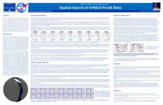
select distinct file_ID, start_date, data_set, ascending_crossing from inventory where data_set like "AVHRR_LAC" and start_date >= 19800101 and end_date <= 20000218 and (ascending_crossing between -80.0 and -64.0) or (ascending_crossing between 88.0 and 106.0) ) 64W 80W 88E 106E Figure 3. Backtrack uses a simplified orbit model to calculate the equatorial crossings for orbits that pass over the area of interest on the ascending (right) and descending (center) passes. The result (right) is a simple, time independent, query. where ( ('2003/02/18 01:23:03' between startDateTime and endDateTime) or ('2003/02/18 03:03:57' between startDateTime and endDateTime) or ('2003/02/18 04:44:34' between startDateTime and endDateTime) or ('2003/02/18 06:05:21' between startDateTime and endDateTime) or ('2003/02/18 07:46:32' between startDateTime and endDateTime) or ('2003/02/18 12:47:46' between startDateTime and endDateTime) or ('2003/02/18 14:10:32' between startDateTime and endDateTime) or ('2003/02/18 15:51:02' between startDateTime and endDateTime) or ('2003/02/18 17:11:31' between startDateTime and endDateTime) or ('2003/02/18 18:52:07' between startDateTime and endDateTime) ) National Snow and Ice Data Center Spatial Search of Orbital Swath Data swick@nsidc.org, knowlesk@nsidc.org Ross S. Swick, Kenneth W. Knowles Abstract: Lookup Table Methods: Backtrack Orbit Search: The idea behind lookup table methods is that while spatial search of swath data is difficult, spatial search of other areas, of a different spatial type, isn’t. So, if we can convert the swath into smaller areas that are easier to work with the problem is more manageable. The actual spatial search becomes a preliminary search on the smaller areas in the lookup table, which returns area IDs that match the area of interest. Spatial search of the data is then turned into a search on the set of IDs. The Worldwide Reference System (WRS-1 & WRS-2) used by Landsat is one such method [5]. WRS-1 and WRS-2 are custom coordinate systems based on Landsat orbits. For WRS-1 252 “paths” are defined that correlate with the 252 orbits in the 18-day repeat cycle. Then, each path is broken into 248 “rows” that each represent 25 seconds, or about 1.45 degrees, of coverage in the path. This scheme yields 62,496 areas to search on in the lookup table and each Landsat scene in the inventory is tagged with the path and row coordinates it covers. The path and row coordinate system is similarly defined for WRS-2 based on a shorter 16-day repeat cycle. The Nominal Orbit Spatial Extent (NOSE) scheme used by NASA’s Earth Observing System (EOS) is an attempt to extend the WRS concept to other satellites and other sensors [2]. For satellites without a well defined and enforced repeat cycle, a typical implementation of NOSE will simply create 360 nominal orbits, one per degree, called “tracks”. Each track will then be broken into 36 “blocks” that each represents about 2.7 minutes, or 10 degrees, of coverage in the track. This scheme yields 12,960 smaller areas to search on in the lookup table and each granule in the inventory is tagged with the track and block coordinates it covers. The high volume of today's remotely sensed Earth Science data creates a strong motivation to minimize the amount of data delivered to the end user. The goal is to get users everything they need but nothing they don't need. One way to decrease the amount of unneeded data delivered is to increase spatial search accuracy. Unfortunately, the most voluminous data, orbital swath data, is also the most difficult to run spatial searches on. Three reasonably accurate means for spatially searching orbital swath data are: methods employing lookup tables, methods employing orbit propagators, and backtrack orbit searching. This paper outlines these three types of methods and discusses some of the advantages and disadvantages of each. The Backtrack Orbit Search Algorithm (BOSA) is currently in use at the National Snow and Ice Data Center (NSIDC) and NASA’s EOS ClearingHOuse (ECHO). The idea behind backtrack orbit search is that while spatial search of swath data is difficult in general, Earth Science swath data has a number of characteristics that make the task a lot easier. Remotely sensed data is valuable to Earth scientists because it is frequent, regular, and global. For the purposes of doing Earth Science, scientists have an interest in keeping the data as consistent as possible. Among other things, that means they want the sensor to have a constant field of view. An easy way to accomplish that is to put the satellite in a circular orbit. For this reason (and others), all Earth Science satellites are in a circular orbit. The Backtrack Orbit Search Algorithm [4] exploits this fact to greatly simplify the orbit model by just modeling an orbit as a great circle under which the Earth rotates. The simplicity of the model allows backtrack to be more efficient than orbit propagator methods, which are designed to work with any satellite. The simplified orbit model relies on only three parameters: inclination, period, and swath width. The accuracy of the method depends on the stability of those three parameters over the life of the sensor, but there is also a scientific interest in keeping those parameters stable, so they generally stay within reason, or the data aren’t useful. As the name implies, backtrack works by tracing the orbit backwards. Backtrack starts with the area of interest and answers the question “In order for the sensor to have seen this area, where must the satellite have crossed the equator?” There is no time dependence, so the speed of the algorithm is independent of the time range searched. There is no cumulative error because backtrack backs up at most one orbit. There is no performance hit from using a lookup table because backtrack calculates the actual equatorial crossing range. And, the subsequent search is a simple, fast, boolean search on that crossing range rather than a text search on IDs. Shown below is one such search statement for 20 year’s worth of AVHRR data. Introduction: Many satellites circle the globe, continuously imaging and collecting Earth Science data. These ribbons of remotely sensed data, which wrap around and around the Earth, are called swaths. For convenience, the continuous swaths are split into individual orbits that begin and end where the satellite crosses the equator from south to north. Typical polar orbiting satellites (meaning their orbits go nearly over each pole) will make 14 to 15 orbits per day, with each orbit comprising many megabytes of data. In general, only a few of these orbits will cover a researcher’s study area. Earth scientists requesting data need some means to find these matching orbits. To aid the researcher, most data producers provide spatial search of their inventory. The first problem is to define the area covered by the swath. As provided, most swath data does not contain an explicit description of the covered area. This information is usually computed upon ingest into the database. The simplest and most popular spatial search method is to define both search areas and data coverage areas as latitude, longitude (lat/lon) bounding boxes on a flat Earth. Latitude and longitude is a common spatial reference system for the Earth and all swath data users should be familiar with its use. (All methods discussed here are projection neutral.) A lat/lon bounding box simplifies spatial search because each area can be completely defined with only four numbers and area intersections can be determined by appropriate boolean comparisons of the minima and maxima. The popularity of this method is understandable because it’s easy to implement and sufficient for most purposes. Orbital swath data is an extraordinarily bad fit to a lat/lon bounding box. A single orbit swath from a sensor with a sufficiently wide field of view can easily cover all latitudes and all longitudes while covering only a small portion of the Earth. Spatial search of orbital swath data requires special methods to accurately and efficiently compare search areas to data coverage areas. Because both WRS and NOSE rely on custom coordinate systems derived from the orbital characteristics of the satellite and the field of view of the sensor, they end up being sensor specific schemes. This means the work involved in creating the lookup table in the first place has to be repeated for each new sensor, and sometimes even for the same sensor on a different satellite. A more general approach is to break the Earth into areas that are independent of the data being collected. A simple approach is to use 1x1 degree lat/lon bins, which yields 64,800 smaller areas to search on in the lookup table. Because those bins are generic the lookup table can be reused for swath data from other sensors, and even for other kinds of data. Indeed, one advantage of a binning scheme is that it can be used for all types of data, which means the data provider can have a single spatial search mechanism for all its data. Both accuracy and performance will suffer as a result, but the trade-off may be worth it in some cases. Lookup table schemes all require some preprocessing of the data to determine which IDs each granule in the inventory should be tagged with. But, the main disadvantage is both accuracy and performance suffer. Landsat has an advantage in that the orbit is tightly controlled and any drift in the satellite is periodically corrected. So, even with only 252 paths defined, the accuracy is much better than the (360/252=) 1.43 degrees one would expect. Moreover, the performance hit associated with using the lookup table in a preliminary search can often be avoided because Landsat users have become so accustomed to the WRS scheme they often search directly on the path and row coordinates they already know cover their area of interest. Satellites in less tightly controlled orbits must rely on the more general NOSE scheme or a simple binning scheme. With 360 nominal orbits defined, or bins defined as 1x1 degree boxes, accuracy is limited to 1 degree, or 111 km at the equator. Greater accuracy requires a larger lookup table, which further degrades performance. There are schemes that use bins of variable size, hierarchical nesting, and more efficient search methods, for example, Peano keys, Morton codes, R-trees, spherical quad-trees, etc., which may partially mitigate the performance issues. However these schemes require the swath coverage to be computed, either by a lat/lon bounding box, nominal orbit, or orbit propagator. We have already discussed the problems with the lat/lon bounding box. Once you have found a nominal orbit or defined the coverage with an orbit propagator, as we shall see, it’s no longer an area comparison problem. The main disadvantage of backtrack is that the crossings do have to be in the database to be searched on. Those values are generally known but because they are not generally used they don’t often get stored in the database. So, a change to the inventory table will usually be required. Orbit Propagator Methods: Summary: Orbit propagators have been around for quite a while because they are useful for more than just spatial search. They are primarily used to simply track and predict satellite movements and using them for search purposes evolved naturally from that. Systems that use propagators to run spatial search include: NOAA’s Comprehensive Large Array-data Stewardship System (CLASS), The University of Wisconsin-Madison’s Man computer Interactive Data Access System (McIDAS), and The University of Alabama-Hunstville’s Space Time Toolkit (STT). The idea behind using orbit propagator methods for spatial search is that while spatial search of swath data is difficult, temporal search isn’t. Orbit propagators work by using an orbit model to determine when the satellite was over the area of interest [1]. Given a time range for the search the propagator will initialize with an ephemeris file that defines exact position, speed, and heading of the satellite prior to the start of the time range. The propagator then spins the model forward to predict when the sensor saw the area of interest. Any cumulative error is corrected by periodically re-initializing the system with known ephemeris data. Consequently the spatial search is turned into a temporal search and since the temporal coverage of each granule is already in the inventory table no database changes are required. Once an orbit propagator is integrated into a system the addition of new satellites, and new sensors, is relatively easy. Because they use actual ephemeris data and reinitialize periodically, orbit propagators can be quite accurate. Because they turn spatial search into temporal search, orbit propagators are ideally suited for use in coincident search. And, both the work of the propagator and the subsequent search are fast enough for short time ranges that performance is not an issue. The main disadvantage of orbit propagator methods is that performance is inversely related to the time range searched. Earth scientists studying climate change are often interested in data over a time range of several years or even decades and at these time scales performance drops dramatically. No matter how fast the propagator may be it still has to spin through the entire time range, which means the time it takes the propagator to complete its task is directly proportional to the time range searched. More importantly, the end result is a large set of disjoint time ranges to search on, which can degrade database performance considerably. For example, Thule, Greenland is located fairly far north and sensors on board polar orbiting satellites see Thule frequently. Many sensors see Thule ten times a day, which results in a query for a single day’s worth of data like the one below. A request for a year’s worth of data over Thule would result in 3,650 disjoint time ranges to search on. Obviously, the problem is less extreme at lower latitudes where coverage is less frequent. But, even at a point near the Equator, where coverage may be only twice daily, a request for only a year’s worth of data would result in a search on 730 disjoint time ranges Lookup table methods provide reasonably fast search once the table parameters are defined, calculated, and stored in the database. New satellites or sensors require new parameter schemes. Both search speed and accuracy are determined by the size of the individual bins in the table. Orbit propagator methods are the most accurate means of searching. However, the search speed is proportional to the length of the time interval of interest. This penalty is paid twice, once in building the query, and once in executing the search. The ancillary ephemeris data is unique to each satellite and requires frequent updating. Backtrack orbit searching is fast and accurate. However, it is restricted to sensors with a constant field of view on satellites in circular orbits. The ancillary orbit parameters are unique to each satellite and sensor, but only need be obtained one time. Accuracy depends on the stability of those parameters. The crossing times must be added to the database. Throughout this paper we have assumed single orbit granules. Each of the methods described requires some adjustment for partial or multiple orbit granules—some more than others. The choice of which method to use largely depends on the purpose of the system. For the purposes of searching inventories of orbital Earth Science data we highly recommend backtrack as faster, cheaper, and more efficient than any other method. Moreover, the accuracy of backtrack orbit search is competitive with orbit propagator methods without the attendant performance issues. We realize this is a qualitative analysis. Further quantitative tests need to be done. References: [1] Bates, Roger R., Donald D. Mueller, and Jerry E. White, Fundamentals of Astrodynamics, Dover Publications, New York, 1971. [2] Heroux, David. "Leveraging Nominal Orbit Spatial Extent to Provide a Solution for the Archival of Geoscience Laser Altimeter System (GLAS) Products in ECS",, December, 2001. [3] Swick R. and K. Knowles, “Spatial Tools for a Round Planet”, Poster #OS51B-166 at the American Geophysical Union Fall Meeting, San Francisco, December 6-10, 2002. [4] Swick, R., and K. Knowles. "The Backtrack Orbit Search Algorithm", http://www.geospatialmethods.org/bosa, November, 2004. [5] Williams, Daryl. "The Worldwide Reference System (WRS)", http://landsat.gsfc.nasa.gov/documentation/wrs.html, May, 2004. Figure 2. A typical satellite orbits the Earth 14 times a day and a typical sensor might see Thule on 10 of those orbits. The resulting temporal clause created by an orbit propagator to search for data over Thule on February 18, 2003 is shown at the right.