Download
1 / 31
310 likes | 482 Views
Why almost all k - c o l o r a b l e graphs are easy ?. A. Coja-Oghlan, M. Krivelevich, D. Vilenchik. Talk Outline. Random graphs: phase transitions and clustering How do typical k -colorable graphs look? Efficient algorithm for coloring k -colorable graphs

E N D
Why almost all k-colorable graphs are easy ? A. Coja-Oghlan, M. Krivelevich, D. Vilenchik
Talk Outline • Random graphs: phase transitions and clustering • How do typical k-colorable graphs look? • Efficient algorithm for coloring k-colorable graphs • Message passing and clustering (SAT)
The k-Coloring Problem Given a graph G=(V,E): • Find f :V! [k] s.t. 8(u,v)2E(G):f(u)f(v) • Find f with minimal possiblek • Such k is called the chromatic number of G, (G) • E.g. (G)=3 1 2 4 3
The k-Coloring Problem • Finding a k-coloring is NP Hard • No polynomial time algorithm approximates(G) within factor better than n1- (unless NPµZPP) [FK98] • How to proceed? random models and average case analysis • Gn,p- every possible edge is included w.p. p=p(n) • (Gn,p)=np/2ln(np) for np2[c0,n/log7n] [Bol88,Luc91]
Phase transitions and clustering • Consider the variant Gn,mofGn,p: • Choose uniformly at random m=m(n) edges • When m=p¢choose(2,n) - Gn,mandGn,p are “close” • There exists a constant d=d(k) such that • 2m/n>d: almost all graphs in Gn,marenot k-colorable • 2m/n<d: almost all graphsare k-colorable [Fri99] • Such phenomena is called a phase transition
Phase transitions and clustering • Gn,m with 2m/n just below the threshold is “hard” experimentally • Possible explanation (partially non-rigorous) comes from statistical physics [MPWZ02] • The “geometrical” structure of the space of proper k-colorings - the clustering phenomena • Need to define notion of distance
Phase transitions and clustering • Two k-colorings are the same if they differ only by a permutation of the color classes • Two k-colorings , are at distancet if • they disagree on the color of at least t vertices in every permutation of the color classes. • There exists one permutation obtaining equality Similar to Hamming distance
Phase transitions and clustering Gn,m with 2m/n just below the threshold: based on analysis that uses partially-rigorous tools • All colorings within a • cluster are “close” • A linear number of • vertices are “frozen” • Proved rigorously for k-SAT, k¸8 [AR06,MMZ05,MMZ05] • For k-SAT: not believed to be true for small k, say k=3 • [MMW05] • Every two clusters are “far” • from each other • Exponentially many clusters
Phase transitions and clustering Why does this structure make life hard? • Heuristics get “distracted” by this structure • Every cluster “pulls” in its direction • Heuristics try to find a compromise between clusters • This is impossible due to the structure • Survey Propagation does well in practice [BMWZ05]
V1 V2 V3 Random k-colorable graphs • Gn,m with 2m/n above the threshold – not suitable to study k-colorable graphs • Instead, consider Gn,m | { k-colorability } • The uniform distribution over k-colorable graphs with exactly m edges • Another possibility, the planted modelGn,m,k • Partition the vertex set into k color classes of size n/k • Include m random edges that respect the coloring
Our Results • Characterization of Gn,m | { k –colorability } • 2m/n=Ck, Cka sufficiently large constant • Using rigorous analysis we show that typically: • Single cluster of proper k-colorings • Size of the cluster is exponential in n • (1-exp{-(Ck)})n vertices are “frozen”
Our Results • There exists a deterministic polynomial time algorithm that k-colors almost all k-colorable graphs with m>Ckn edges. Cka sufficiently large constant. • Rigorously complement results for sparse case: • When clustering is simple – the problem is easy • When clustering is “complicated” – the problem is harder (?) Almost all k-colorable graphs are easy !
Our Results • Show that Gn,m,k and Gn,m | { k –colorability } share many structural properties (“close”) • Justifying the somewhat unnatural usage of planted-solution models • Alon-Kahale’s coloring algorithm [AK97] works for Gn,m | { k –colorability } as well • Gn,m,k also has the same clustering structure
Our Results • Our results also apply to thek-SAT setting • Similar threshold and clustering phenomena are known/believed for k-SAT • The planted and uniform SAT distributions are “close” • Flaxman’s algorithm for planted 3CNF formulas works for the uniform setting • Improving the exponential time algorithm for uniform satisfiable 3CNFs (only one known so far) • Answering open research questions in [BBG02]
V1 V2 V3 Clustering: Proof Techniques • Recall, Gn,m | { k-colorability } • The uniform distribution over k-colorable graphs with exactly m edges • Why more difficult than the planted distribution? • Edges are notindependent • For starters, consider the planted distribution Gn,p,k (k=3)
Proof Techniques – The Core • Every vertex is expected to have d/3 neighbors in every other color class (d=np) Claim 1: whp there is no subgraph H of G s.t. |V(H)|<n/100 and E(H)>d|H|/10 d¸d0, d0 a sufficiently large constant Claim 2: whp there are no two proper 3-colorings at distance greater than n/100
V1 V2 V3 Proof Techniques – The Core Claim 3: Suppose that every vertex has the expected degree, and Claims 1 and 2 hold. Then the graph G is uniquely 3-colorable. Proof: - the planted coloring. If not unique, 9, dist(,)<n/100(Claim 1). U - set of disagreeing vertices. (v)(v) )v has d/3 neighbors in U. |U|<n/100, |E(U)|>d|U|/6 – Contradicting Claim 2.
Proof Techniques – The Core • This is whp the case when np > Ck log n • When np=O(1) – whp not the case • Definition of Core H : v2H if • v has at least np/4 neighbors in G[H] in • every other color class • v has at most np/10 neighbors outside of H. • Claim 4: 9 Core H s.t. whp • |H | ¸ (1-exp{-(np)})n • H is uniquely 3-colorable
V1 V2 V3 Proof Techniques – The Core Corollary: • (1-exp{-(np)})n vertices are frozen in every proper 3-coloring • Only one cluster of exponential size V1 V2 V3
Moving to the Uniform Case • A – a “bad” graph property (e.g. the graph has no big core) • – the expected number of proper k-colorings of random graph in the planted distribution Claim 5: Pruniform[A] ·¢Prplanted[A] Intuition: typically there are at most ways to generate G in the planted model. Now use a union bound.
Moving to the Uniform Case • A – “the graph has no big core” Claim 6: Prplanted[A] · e-exp{-C1}n There exists no proper 3-coloring w.r.t which there exists a big core Claim 7: · eexp{-C2}n, C2 > C1 Corollary: Pruniform[A] = o(1)
Algorithmic Perspective • Show that Alon and Kahale’s algorithm [AK97] works in the uniform case • What is Alon and Kahale’s algorithm? • Approximate a proper 3-coloring (spectral techniques) • Refine the coloring – recoloring step • Uncolor “suspicious” vertices • G[U] – graph induced by uncolored vertices • Exhaustively color G[U] according to G[V\U] Outcome differs from planted on n/1000 vertices Outcome agrees on the core • Core remains colored • Every colored vertex • agrees with planted Logarithmic size connected components
Algorithmic Perspective - Analysis • Typically, uniform graphs have a big core • Two more facts needed for the analysis: • Claim 1 in the uniform case • Logarithmic size components in G[V \ H] • Both properties hold w.p. 1-1/poly(n) in the planted model - cannot use “union bound” • Solution: analyze directly the uniform distribution • Difficulty: edges are strongly dependent • Solution: careful, non-trivial, counting argument
Algorithmic Perspective - SAT • Show that Flaxman’s algorithm [Fla03] works in the uniform case • What is Flaxman’s algorithm? • Approximate a satisfying assignment (majority vote) • Unassign “suspicious” variables • G[U] – graph induced by unassigned variables • Exhaustively satisfy G[U] according to G[V \ U]
SAT and Message Passing Warning Propagation: • Given a formula F – define Factor Graph G(F) • Bipartite graph: V1 = variables, V2 = clauses • (x,C)2E(G) iff x appears in C • Two types of messages: C=(xÇyÇz) • Cx = 1 if yC < 0 and zC < 0; 0 otherwise • xC = (x2 C’,C’C C’x) – (¬x2 C’’C’’x)
SAT and Message Passing • WP(F) • Repeat until no message changes: • Initialize all messages Cx to 1/0 w.p. 0.5 • Randomly order the edges of G(F) • Evaluate all messages Cx • Assign every x according to (x2 C’C’x) – (¬x2 C’’C’’x) • Theorem [FMV06]: If F sampled according to Planted 3SAT • p=d/n2,d sufficiently large constant, then whp: • WP converges after O(log n) iterations • Assigned variables agree with some satisfying assignment • All but exp{-(d)}n variables are assigned • Clauses of unassigned variables are “easy” to satisfy
SAT and Message Passing • Our work implies – [FMV06] applies for the uniform SAT setting as well • Reinforces the following thesis: • When clustering is complicated) formulas are hard) sophisticated algorithms needed: Survey Propagation • When clustering is simple) formulas are easy) naïve algorithms work: Warning Propagation
Further Research • Loose • Rigorouslyanalyze Survey Propagation on near-threshold formulas/graphs • First step – analyze Survey Propagation on Planted instances • Prove the near-threshold clustering phenomena • Rigorously analyze message passing algorithms • Analyze instances with an arbitrary constant (above the threshold) density