Download
1 / 38
380 likes | 474 Views
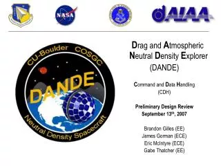
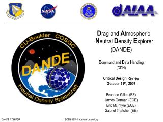
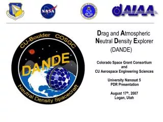
D rag and A tmospheric N eutral D ensity E xplorer (DANDE ) Colorado Space Grant Consortium and CU Aerospace Engineering Sciences COSGC Symposium April 20, 2013 Boulder, Colorado. Over-View of the DANDE Spacecraft and science instruments.

E N D
Drag and Atmospheric NeutralDensity Explorer (DANDE) Colorado Space Grant Consortium and CU Aerospace Engineering SciencesCOSGC SymposiumApril 20, 2013Boulder, Colorado
Over-View of the DANDE Spacecraft and science instruments. Discussion of time offset measurement algorithm. Discussion of ACC data processing algorithms. Emphasis will be placed on these two specifics aspects of the DANDE Mission Outline
DANDE Mission DRAG and ATMOSPHERIC NEUTRAL DENSITY EXPLORER Mission Statement Explore the spatial and temporal variability of the neutral thermosphere at altitudes of 350 - 200 km, and investigate how wind and density variability translate to drag forces on satellites.
DANDE Mission DRAG and ATMOSPHERIC NEUTRAL DENSITY EXPLORER Mission Statement Explore the spatial and temporal variability of the neutral thermosphere at altitudes of 350 – 200 325 - 1500km, and investigate how wind and density variability translate to drag forces on satellites.
Operational Importance of Drag The density of the atmosphere in this region varies greatly (300% to 800%*) due to space weather and not yet understood coupled processes. 410 km X5 flare7/14/2000 390 km 370 km decay reboost 350 km ISS drops 10kmin several days 330 km 2000 2001 1999 E. Semones et.al. WRMISS 10 http://www.oma.be/WRMISS/workshops/tenth/pdf/ex02_semones.pdf • Forbes et. Al. “Thermosphere density response to the 20-21 November 2003 solar and geomagnetic storm from CHAMP and GRACE accelerometer data”, Journal of Geophysical Research, Vol. 111, June 2006 • European Space Agency Debris Tracking
Operational Importance of Drag The density of the atmosphere in this region varies greatly (300% to 800%*) due to space weather and not yet understood coupled processes. • Forbes et. Al. “Thermosphere density response to the 20-21 November 2003 solar and geomagnetic storm from CHAMP and GRACE accelerometer data”, Journal of Geophysical Research, Vol. 111, June 2006 • European Space Agency Debris Tracking
Satellite Drag CHAllengingMinisatellite Payload Satellite drag measurements suffer from errors caused by • Unknown acceleration contribution from in-track winds • coefficient of drag accuracy DANDE is designed to address these issues and provide acceleration, composition, and wind measurements simultaneously along with a well determined drag coefficient at ~350 km Starshine I
How Measurements are Made Identifying all components of the constituents of the drag equation. With a near-spherical shape, an a-priori physical drag coefficient may be calculated and a physical density can be obtained from the measurements A atmosphere ρ - density VW FD V CD tracking WTS sensor accelerometers solution a priori knowledge a priori knowledge a priori knowledge comparison solved 8
Dual Instrument Approach 1/6 Hz drag signal Measured Energy Spectrum Frequency [Hz]
Acceleration Measurements • Accelerometer Sensor Heads • QA-2000 X 6 Units • Phased by 60° • Analogue Filtering • 4th Order Bandpass • 0.05-0.5Hz • 60dB Gain in the bandpass • High Pass removes centripetal acceleration • Low Pass removes intrinsic noise • Each ACC head filtered independently • ADC acts as 6 independent accelerometers in one package • Simultaneous sampling of each ACC head
Low frequency bias spin rate ANALOG FILTERING DATA FITTING A/D CONVERSION 70 ng Acceleration Measurements
ACC-2 ACC-4 ACC-1 ACC-6 ACC-3 ω ACC-5 Acceleration Measurements FD
Acceleration Measurements • Atmosphere Sample Enters from the left • Collimator rejects natural ions, leaving only neutral particles • Ionizing filament ionizes the neutral particle stream • SDEA deflects the now charged atmosphere constituents a variable amount (depending on ramp voltage)
channel 1 channel 2 ..... channel 7 channel 8 channel 9 channel 10 channel 11 channel 12 NMS: Angular Distribution Schematic Ionizer Small Deflection Energy Analyzer Collimator
NMS Data Product • Energy of each particle is used to give the velocity at which that particle entered the instrument • Spread in each peak gives a measure of the temperature of the constituent • Displacement from the center anode gives the wind angle (as illustrated previously)
Time Mapping 19
Time Mapping • WHAT is TOM? • Program written in order to accurately calculate and place a time on downlinked data • WHY do we need TOM? • DANDE does not have GPS • DANDE system reset DANDE system time set back to 1/1/1970 at 12:00 a.m. • Need to ‘map’ DANDE system time to local time on ground in order to have accurate and usable science data
Time Mapping • How are Time Offset Measurements Taken? • Mission operators send “MeasureTimeOffset” command from InControl client to DANDE satellite • Command asks for current time on DANDE satellite • Sends this information to ground server • Time elapsed since sent command is called “command time” • Assume DANDE time measurement occurred at half of the “command time” • Process repeated 5 times to attain necessary accuracy
Time Mapping • HOW can we use TOM? • Fine Time Mapping: to the units of micro-seconds, needs two time offset measurements from two separate passes, epoch needs to be mapped to ground time • Necessary for science modes • Coarse Time Mapping: to the units of seconds, epoch needs to be mapped to ground time • Emergency Time Mapping: to the units of minutes, no time offset measurements, only for Health and Status files
Time Mapping • Verify epoch needed for processing has recorded ground start time • No entry: Run EpochStartCalculator.m • Enter epoch information into epochstart.csv • epochStart.csv has ground starting times of all epochs • Run TimeOffsetMeasurementChecker.m • Tells us how many T.O.M.’s accumulated for a given epoch, will recommend fine or coarse time mapping • Also use operator’s discretion on fine, coarse, or emergency – depends on which subsystem you are processing data for • FINE/ COARSE • Execute ProcessedDownlinkedFiles command on InControl
Time Mapping • EMERGENCY: • Used when data processing (H&S files) is crucial during a pass, and no time offset measurements have been accumulated • Two options for mapping an epoch start time: • Error Logs record DANDE time right before a reset • Requires a manual calculation: (DANDE ground time from last T.O.M.)–(Ground Time right before DANDE reset/ Epoch Start Time) = DANDE present time • Health and Status files record epoch and DANDE time • Epoch start time requires a manual calculation: (Ground time) - (DANDE time) = Epoch Start Time (ground) • Once epoch start time is recorded, can proceed to processing data
ACC Data Inversion • Back out the filtering and amplification. This has to be done assuming an ideal band pass • The signal is then converted to an acceleration using honey-well provided temperature curves • Temperature compensation is also applied to each analog filter string.
ACC Data Inversion • The actual data product of interest in the density of the environment • Blue labeled parameters are either modeled or measured prior to launch • Green parameters are either modeled, or measured by NMS • The force is the desired product from ACC, being manifested as the amplitude of the drag signal
ACC Data Characteristics • We have previously used the signals periodicity for analog processing. • How else can we use this to better improve the data resolution?
ACC Data Characteristics • Potential algorithms utilizing this feature
ACC Direct LSF Fit • Treats each accelerometer independently • Allows for each string to be compared • Simple and relatively easy • Well defined fit uncertainty
ACC Coupled LSF Fit • Takes each string, and applies a phase shift such that each signal is the same • Signals are then summed, giving a single sinusoid, with amplitude 6 times the original signal • In certain situations (very low signal to noise ratio) improves the co-efficient uncertainty from the LSF
ACC Coupled LSF Fit • This data was simulated with added Gaussian noise of the same amplitude, and variance 50% of the signal amplitude. • The singular fit gives a 42% uncertainty in amplitude • The coupled fit provides a 17% uncertainty in fit parameter
ACC Very Noisy Data • With the current orbit DANDE will be outside the designed density for a substantial amount of time • To account for this a developed system for pulling parameters from extremely noisy data • The simulated data has a noise variance twice that of the signal amplitude. The amplitude here is 2.
ACC Very Noisy Data • The LSF programs, coupled or singular, are unable to fit to this data
ACC Fourier Based Filtering • When filtered through an FFT algorithm, we can see that the signal frequencies are still dominant in the signal • We can take advantage of this by isolating just the signal we want, which will have a well defined frequency based on the spin rate of the satellite.
ACC Fourier Based Filtering • Filter is applied digitally, simply setting all frequency components outside of a window around the dominant frequency to zero • When passed back through an inverse transform we obtain the original signal, with aberrations around the edges from the distortion of the filtering
Conclusion • Provides a novel approach to characterization of the atmosphere of low earth orbit • TOM correlates DANDE’s system time to the local ground time which allows time mapping to varying degrees of accuracy • Forced drag signal modulation enables enhanced on board filtering, and improved data fitting techniques.
Drag and Atmospheric NeutralDensity Explorer Questions? Winner of University Nanosat V Competition