Download
1 / 19
220 likes | 460 Views
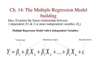
Ch. 14: The Multiple Regression Model building. Idea: Examine the linear relationship between 1 dependent (Y) & 2 or more independent variables (X i ). Multiple Regression Model with k Independent Variables:. Population slopes. Random Error. Y-intercept. Estimated (or predicted)

E N D
Ch. 14: The Multiple Regression Model building Idea: Examine the linear relationship between 1 dependent (Y) & 2 or more independent variables (Xi) Multiple Regression Model with k Independent Variables: Population slopes Random Error Y-intercept
Estimated (or predicted) value of Y Estimated intercept Estimated slope coefficients • The coefficients of the multiple regression model are estimated using sample data with k independent variables • Interpretation of the Slopes: (referred to as a Net Regression Coefficient) • b1=The change in the mean of Y per unit change in X1, taking into account the effect of X2 (or net of X2) • b0 Y intercept. It is the same as simple regression.
Graph of a Two-Variable Model • Three dimension Y Slope for variable X1 X2 Slope for variable X2 X1
Example: • Simple Regression Results • Multiple Regression Results • Check the size and significance level of the coefficients, the F-value, the R-Square, etc. You will see what the “net of “ effects are.
Using The Equation to Make Predictions • Predict the appraised value at average lot size (7.24) and average number of rooms (7.12). • What is the total effect from 2000 sf increase in lot size and 2 additional rooms?
Coefficient of Multiple Determination, r2 and Adjusted r2 • Reports the proportion of total variation in Y explained by all X variables taken together (the model) • Adjusted r2 • r2 never decreases when a new X variable is added to the model • This can be a disadvantage when comparing models
What is the net effect of adding a new variable? • We lose a degree of freedom when a new X variable is added • Did the new X variable add enough explanatory power to offset the loss of one degree of freedom? • Shows the proportion of variation in Y explained by all X variables adjusted for the number of Xvariables used (where n = sample size, k = number of independent variables) • Penalize excessive use of unimportant independent variables • Smaller than r2 • Useful in comparing among models
Multiple Regression Assumptions • Assumptions: • The errors are normally distributed • Errors have a constant variance • The model errors are independent • Errors (residuals) from the regression model: ei = (Yi – Yi) • These residual plots are used in multiple regression: • Residuals vs. Yi • Residuals vs. X1i • Residuals vs. X2i • Residuals vs. time (if time series data)
Y Two variable model Sample observation Yi Residual = ei = (Yi – Yi) < Yi < x2i X2 x1i < The best fit equation, Y , is found by minimizing the sum of squared errors, e2 X1
Are Individual Variables Significant? • Use t-tests of individual variable slopes • Shows if there is a linear relationship between the variable Xi and Y; Hypotheses: • H0: βi = 0 (no linear relationship) • H1: βi≠ 0 (linear relationship does exist between Xi and Y) • Test Statistic: • Confidence interval for the population slope βi
Is the Overall Model Significant? • F-Test for Overall Significance of the Model • Shows if there is a linear relationship between all of the X variables considered together and Y • Use F test statistic; Hypotheses: H0: β1 = β2 = … = βk = 0 (no linear relationship) H1: at least one βi≠ 0 (at least one independent variable affects Y) • Test statistic:
Testing Portions of the Multiple Regression Model • To find out if inclusion of an individual Xj or a set of Xs, significantly improves the model, given that other independent variables are included in the model • Two Measures: • Partial F-test criterion • The Coefficient of Partial Determination
Contribution of a Single Independent Variable Xj SSR(Xj | all variables except Xj) = SSR (all variables) – SSR(all variables except Xj) • Measures the contribution of Xj in explaining the total variation in Y (SST) • consider here a 3-variable model: SSR(X1 | X2 and X3) = SSR (all variablesX1-x3) – SSR(X2 and X3) SSRR Model SSRUR Model
The Partial F-Test Statistic • Consider the hypothesis test: H0: variable Xj does not significantly improve the model after all other variables are included H1: variable Xj significantly improves the model after all other variables are included Note that the numerator is the contribution of Xj to the regression. If Actual F Statistic is > than the Critical F, then Conclusion is: Reject H0; adding X1 does improve model
Coefficient of Partial Determination for one or a set of variables • Measures the proportion of total variation in the dependent variable (SST) that is explained by Xj while controlling for (holding constant) the other explanatory variables
Using Dummy Variables • A dummy variable is a categorical explanatory variable with two levels: • yes or no, on or off, male or female • coded as 0 or 1 • Regression intercepts are different if the variable is significant • Assumes equal slopes for other variables • If more than two levels, the number of dummy variables needed is (number of levels - 1)
Fire Place No Fire Place • Different Intercepts, same slope Fire Place (X2 = 1) Y (sales) If H0: β2 = 0 is rejected, then “Fire Place” has a significant effect on Values b0 + b2 No Fire place (X2 = 0) b0
Interaction Between Explanatory Variables • Hypothesizes interaction between pairs of X variables • Response to one X variable may vary at different levels of another X variable • Contains two-way cross product terms • Effect of Interaction • Without interaction term, effect of X1 on Y is measured by β1 • With interaction term, effect of X1 on Y is measured by β1 + β3 X2 • Effect changes as X2 changes
= 1 + 2X1 + 3X2 + 4X1X2 • Example: Suppose X2 is a dummy variable and the estimated regression equation is Y X2 = 1: Y = 1 + 2X1 + 3(1) + 4X1(1) = 4 + 6X1 X2 = 0: Y = 1 + 2X1 + 3(0) + 4X1(0) = 1 + 2X1 X1 0 0.5 1 1.5 Slopes are different if the effect of X1 on Y depends on X2 value