Download
1 / 119
2.05k likes | 4.52k Views
Assumptions of multiple regression. Assumption of normality Assumption of linearity Assumption of homoscedasticity Script for testing assumptions Practice problems. Assumptions of Normality, Linearity, and Homoscedasticity.

E N D
Assumptions of multiple regression Assumption of normality Assumption of linearity Assumption of homoscedasticity Script for testing assumptions Practice problems
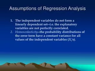
Assumptions of Normality, Linearity, and Homoscedasticity • Multiple regression assumes that the variables in the analysis satisfy the assumptions of normality, linearity, and homoscedasticity. (There is also an assumption of independence of errors but that cannot be evaluated until the regression is run.) • There are two general strategies for checking conformity to assumptions: pre-analysis and post-analysis. In pre-analysis, the variables are checked prior to running the regression. In post-analysis, the assumptions are evaluated by looking at the pattern of residuals (errors or variability) that the regression was unable to predict accurately. • The text recommends pre-analysis, the strategy we will follow.
Assumption of Normality • The assumption of normality prescribes that the distribution of cases fit the pattern of a normal curve. • It is evaluated for all metric variables included in the analysis, independent variables as well as the dependent variable. • With multivariate statistics, the assumption is that the combination of variables follows a multivariate normal distribution. • Since there is not a direct test for multivariate normality, we generally test each variable individually and assume that they are multivariate normal if they are individually normal, though this is not necessarily the case.
Assumption of Normality:Evaluating Normality There are both graphical and statistical methods for evaluating normality. • Graphical methods include the histogram and normality plot. • Statistical methods include diagnostic hypothesis tests for normality, and a rule of thumb that says a variable is reasonably close to normal if its skewness and kurtosis have values between –1.0 and +1.0. • None of the methods is absolutely definitive. • We will use the criteria that the skewness and kurtosis of the distribution both fall between -1.0 and +1.0.
Assumption of Normality:Histograms and Normality Plots On the left side of the slide is the histogram and normality plot for a occupational prestige that could reasonably be characterized as normal. Time using email, on the right, is not normally distributed.
Assumption of Normality:Hypothesis test of normality The hypothesis test for normality tests the null hypothesis that the variable is normal, i.e. the actual distribution of the variable fits the pattern we would expect if it is normal. If we fail to reject the null hypothesis, we conclude that the distribution is normal. The distribution for both of the variable depicted on the previous slide are associated with low significance values that lead to rejecting the null hypothesis and concluding that neither occupational prestige nor time using email is normally distributed.
Assumption of Normality:Skewness, kurtosis, and normality Using the rule of thumb that a rule of thumb that says a variable is reasonably close to normal if its skewness and kurtosis have values between –1.0 and +1.0, we would decide that occupational prestige is normally distributed and time using email is not. We will use this rule of thumb for normality in our strategy for solving problems.
Assumption of Normality:Transformations • When a variable is not normally distributed, we can create a transformed variable and test it for normality. If the transformed variable is normally distributed, we can substitute it in our analysis. • Three common transformations are: the logarithmic transformation, the square root transformation, and the inverse transformation. • All of these change the measuring scale on the horizontal axis of a histogram to produce a transformed variable that is mathematically equivalent to the original variable.
Assumption of Normality:Computing Transformations • We will use SPSS scripts as described below to test assumptions and compute transformations. • For additional details on the mechanics of computing transformations, see “Computing Transformations”
Assumption of Normality:When transformations do not work • When none of the transformations induces normality in a variable, including that variable in the analysis will reduce our effectiveness at identifying statistical relationships, i.e. we lose power. • We do have the option of changing the way the information in the variable is represented, e.g. substitute several dichotomous variables for a single metric variable.
Assumption of Normality:Computing “Explore” descriptive statistics To compute the statistics needed for evaluating the normality of a variable, select the Explore… command from the Descriptive Statistics menu.
Assumption of Normality:Adding the variable to be evaluated Second, click on right arrow button to move the highlighted variable to the Dependent List. First, click on the variable to be included in the analysis to highlight it.
Assumption of Normality:Selecting statistics to be computed To select the statistics for the output, click on the Statistics… command button.
Assumption of Normality:Including descriptive statistics First, click on the Descriptives checkbox to select it. Clear the other checkboxes. Second, click on the Continue button to complete the request for statistics.
Assumption of Normality:Selecting charts for the output To select the diagnostic charts for the output, click on the Plots… command button.
Assumption of Normality:Including diagnostic plots and statistics First, click on the None option button on the Boxplots panel since boxplots are not as helpful as other charts in assessing normality. Finally, click on the Continue button to complete the request. Second, click on the Normality plots with tests checkbox to include normality plots and the hypothesis tests for normality. Third, click on the Histogram checkbox to include a histogram in the output. You may want to examine the stem-and-leaf plot as well, though I find it less useful.
Assumption of Normality:Completing the specifications for the analysis Click on the OK button to complete the specifications for the analysis and request SPSS to produce the output.
Assumption of Normality:The histogram An initial impression of the normality of the distribution can be gained by examining the histogram. In this example, the histogram shows a substantial violation of normality caused by a extremely large value in the distribution.
Assumption of Normality:The normality plot The problem with the normality of this variable’s distribution is reinforced by the normality plot. If the variable were normally distributed, the red dots would fit the green line very closely. In this case, the red points in the upper right of the chart indicate the severe skewing caused by the extremely large data values.
Assumption of Normality:The test of normality Since the sample size is larger than 50, we use the Kolmogorov-Smirnov test. If the sample size were 50 or less, we would use the Shapiro-Wilk statistic instead. The null hypothesis for the test of normality states that the actual distribution of the variable is equal to the expected distribution, i.e., the variable is normally distributed. Since the probability associated with the test of normality is < 0.001 is less than or equal to the level of significance (0.01), we reject the null hypothesis and conclude that total hours spent on the Internet is not normally distributed. (Note: we report the probability as <0.001 instead of .000 to be clear that the probability is not really zero.)
Assumption of Normality:The rule of thumb for skewness and kurtosis Using the rule of thumb for evaluating normality with the skewness and kurtosis statistics, we look at the table of descriptive statistics. The skewness and kurtosis for the variable both exceed the rule of thumb criteria of 1.0. The variable is not normally distributed.
Assumption of Linearity • Linearity means that the amount of change, or rate of change, between scores on two variables is constant for the entire range of scores for the variables. • Linearity characterizes the relationship between two metric variables. It is tested for the pairs formed by dependent variable and each metric independent variable in the analysis. • There are relationships that are not linear. • The relationship between learning and time may not be linear. Learning a new subject shows rapid gains at first, then the pace slows down over time. This is often referred to a a learning curve. • Population growth may not be linear. The pattern often shows growth at increasing rates over time.
Assumption of Linearity:Evaluating linearity • There are both graphical and statistical methods for evaluating linearity. • Graphical methods include the examination of scatterplots, often overlaid with a trendline. While commonly recommended, this strategy is difficult to implement. • Statistical methods include diagnostic hypothesis tests for linearity, a rule of thumb that says a relationship is linear if the difference between the linear correlation coefficient (r) and the nonlinear correlation coefficient (eta) is small, and examining patterns of correlation coefficients.
Assumption of Linearity:Interpreting scatterplots The advice for interpreting linearity is often phrased as looking for a cigar-shaped band, which is very evident in this plot.
Assumption of Linearity:Interpreting scatterplots Sometimes, a scatterplot shows a clearly nonlinear pattern that requires transformation, like the one shown in the scatterplot.
Assumption of Linearity:Scatterplots that are difficult to interpret The correlations for both of these relationships are low. The linearity of the relationship on the right can be improved with a transformation; the plot on the left cannot. However, this is not necessarily obvious from the scatterplots.
Assumption of Linearity:Using correlation matrices Creating a correlation matrix for the dependent variable and the original and transformed variations of the independent variable provides us with a pattern that is easier to interpret. The information that we need is in the first column of the matrix which shows the correlation and significance for the dependent variable and all forms of the independent variable.
Assumption of Linearity:The pattern of correlations for no relationship The correlation between the two variables is very weak and statistically non-significant. If we viewed this as a hypothesis test for the significance of r, we would conclude that there is no relationship between these variables. Moreover, none of significance tests for the correlations with the transformed dependent variable are statistically significant. There is no relationship between these variables; it is not a problem with non-linearity.
Assumption of Linearity:Correlation pattern suggesting transformation The correlation between the two variables is very weak and statistically non-significant. If we viewed this as a hypothesis test for the significance of r, we would conclude that there is no relationship between these variables. However, the probability associated with the larger correlation for the logarithmic transformation is statistically significant, suggesting that this is a transformation we might want to use in our analysis.
Assumption of Linearity:Correlation pattern suggesting substitution • Should it happen that the correlation between a transformed independent variable and the dependent variable is substantially stronger than the relationship between the untransformed independent variable and the dependent variable, the transformation should be considered even if the relationship involving the untransformed independent variable is statistically significant. • A difference of +0.20 or -0.20, or more, would be considered substantial enough since a change of this size would alter our interpretation of the relationship.
Assumption of Linearity:Transformations • When a relationship is not linear, we can transform one or both variables to achieve a relationship that is linear. • Three common transformations to induce linearity are: the logarithmic transformation, the square root transformation, and the inverse transformation. • All of these transformations produce a new variable that is mathematically equivalent to the original variable, but expressed in different measurement units, e.g. logarithmic units instead of decimal units.
Assumption of Linearity:When transformations do not work • When none of the transformations induces linearity in a relationship, our statistical analysis will underestimate the presence and strength of the relationship, i.e. we lose power. • We do have the option of changing the way the information in the variables are represented, e.g. substitute several dichotomous variables for a single metric variable. This bypasses the assumption of linearity while still attempting to incorporate the information about the relationship in the analysis.
Assumption of Linearity:Creating the scatterplot Suppose we are interested in the linearity of the relationship between "hours per day watching TV" and "total hours spent on the Internet". The most commonly recommended strategy for evaluating linearity is visual examination of a scatter plot. To obtain a scatter plot in SPSS, select the Scatter… command from the Graphs menu.
Assumption of Linearity:Selecting the type of scatterplot First, click on thumbnail sketch of a simple scatterplot to highlight it. Second, click on the Define button to specify the variables to be included in the scatterplot.
Assumption of Linearity:Selecting the variables First, move the dependent variable netime to the Y Axis text box. Third, click on the OK button to complete the specifications for the scatterplot. Second, move the independent variable tvhours to the X axis text box. If a problem statement mentions a relationship between two variables without clearly indicating which is the independent variable and which is the dependent variable, the first mentioned variable is taken to the be independent variable.
Assumption of Linearity:The scatterplot The scatterplot is produced in the SPSS output viewer. The points in a scatterplot are considered linear if they form a cigar-shaped elliptical band. The pattern in this scatterplot is not really clear.
Assumption of Linearity:Adding a trendline To try to determine if the relationship is linear, we can add a trendline to the chart. To add a trendline to the chart, we need to open the chart for editing. To open the chart for editing, double click on it.
Assumption of Linearity:The scatterplot in the SPSS Chart Editor The chart that we double clicked on is opened for editing in the SPSS Chart Editor. To add the trend line, select the Options… command from the Chart menu.
Assumption of Linearity:Requesting the fit line In the Scatterplot Options dialog box, we click on the Total checkbox in the Fit Line panel in order to request the trend line. Click on the Fit Options… button to request the r² coefficient of determination as a measure of the strength of the relationship.
Assumption of Linearity:Requesting r² First, the Linear regression thumbnail sketch should be highlighted as the type of fit line to be added to the chart. Third, click on the Continue button to complete the options request. Second, click on the Fit Options… Click on the Display R-square in Legend checkbox to add this item to our output.
Assumption of Linearity:Completing the request for the fit line Click on the OK button to complete the request for the fit line.
Assumption of Linearity:The fit line and r² The red fit line is added to the chart. The value of r² (0.0460) suggests that the relationship is weak.
Assumption of Linearity:Computing the transformations There are four transformations that we can use to achieve or improve linearity. The compute dialogs for these four transformations for linearity are shown.
Assumption of Linearity:Creating the scatterplot matrix To create the scatterplot matrix, select the Scatter… command in the Graphs menu.
Assumption of Linearity:Selecting type of scatterplot First, click on the Matrix thumbnail sketch to indicate which type of scatterplot we want. Second, click on the Define button to select the variables for the scatterplot.
Assumption of Linearity:Specifications for scatterplot matrix First, move the dependent variable, the independent variable and all of the transformations to the Matrix Variables list box. Second, click on the OK button to produce the scatterplot.
Assumption of Linearity:The scatterplot matrix The scatterplot matrix shows a thumbnail sketch of scatterplots for each independent variable or transformation with the dependent variable. The scatterplot matrix may suggest which transformations might be useful.
Assumption of Linearity:Creating the correlation matrix To create the correlation matrix, select the Correlate | Bivariate… command in the Analyze menu.
Assumption of Linearity:Specifications for correlation matrix First, move the dependent variable, the independent variable and all of the transformations to the Variables list box. Second, click on the OK button to produce the correlation matrix.
Assumption of Linearity:The correlation matrix The answers to the problems are based on the correlation matrix. Before we answer the question in this problem, we will use a script to produce the output.