Download
1 / 38
380 likes | 532 Views
Counting Constraint Satisfaction Problems. Andrei A. Bulatov Simon Fraser University. Dagstuhl 2009. Counting Problems: Graph Reliability. s. t. Every connection fails with probability ½. What is the probability that the two distinguished nodes are connected?.

E N D
Counting Constraint Satisfaction Problems Andrei A. Bulatov Simon Fraser University Dagstuhl 2009
Counting Problems: Graph Reliability s t Every connection fails with probability ½. What is the probability that the two distinguished nodes are connected? # subgraphs in which s and t are connected Prob = # all subgraphs
Counting Problems: Fourier Coefficients Let be a Boolean operation and Fourier coefficient is given by Observe that computing reduces to counting the zeroes of
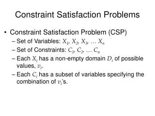
Counting Problems Let L be a problem from NP, and M an NTM solving it. Then the corresponding counting problem is Instance: An instance I of L. Objective: How many accepting paths ofM(I)are there? M(I) This class of problems is called #P
Complexity Classes, Reductions Counting problems solvable in poly time: a subclass of FP Analog of NP: #P Problem A is Turing reducible to problem B if In other words, A can be solved in poly time using B as an oracle Problem A #P is #P-complete if every problem from #P is Turing reducible to A
Complexity Classes Another relevant complexity class: Reconsider the Graph Reliability problem: Every connection fails with probability 1/3. Let the graph have m edge Prob =
Left Side Restrictions #CSP(A,_) counting CSP with left side restricted #CSP(B) or #CSP(B) counting CSP with right side restricted Theorem (Dalmau, Jonsson, 2004) Under certain assumptions from parametrized complexity, for a class of structures A of bounded arity, the problem #CSP(A,_) is solvable in polynomial time if and only if A has bounded treewidth.
#3-SAT = #CSP( ) #k-coloring = #CSP( ) Right Side Restrictions NP-hard (if k 3) (#P-complete) #Linear Equations = #CSP( F ) polytime, FP H is complete bipartite or complete with loops polytime, FP #H-Coloring = #CSP(H) #P-complete (Dyer, Greenhill; 2001) otherwise
More Results #CSP(B)B is a 2-element structure, is solvable in polynomial time if and only if every relation from B can be represented as the set of solutions to a system of linear equations over GF(2). Otherwise it is #P-complete. (N.Creignou, M.Herrman, 1996) #H-Coloring H is an acyclic digraph, is solvable in polynomial time if and only if H satisfies certain conditions; it is #P-complete otherwise (Dyer,Goldberg,Paterson, 2007 )
More Results (cntd) #CSP(S)S corresponds to equations over a finite semigroup, is either solvable in polynomial time, or #P-complete (O.Klima, B.Larose, P.Tesson, )
Two Algorithms: 1 #Linear Equations (over a field F) Algorithm - Find the dimensionality k of the solution space (Gaussian elimination) - Output
i ii I II Two Algorithms: 2 #H-ColoringH is the following digraph
i ii U 2 E 1 4 2 W I II Two Algorithms: 2
PP-Definitions Theorem (B., Dalmau; 2003) If structures B and C are such that every relation of C is pp-definable in B, then #CSP(C) is Turing reducible to #CSP(B)
a b c x a z b c y PP-Definitions (cntd) Running example: H = (V; E) Relational product E E(x,y) = zE(x,y) E(z,y)
a b c x y z PP-Definitions (cntd) Another example
CSP(B), CSP(C), and CSP( ) are poly-time reducible to CSP(A) #CSP(B), #CSP(C), and #CSP( ) are Turing reducible to #CSP(A) Algebraic Theory: Polymorphisms If Pol(A) Pol(B), then CSP(B) is poly-time reducible to CSP(A) If Pol(A) Pol(B), then #CSP(B) is Turing reducible to #CSP(A)
Algebraic Theory: Varieties If CSP(A) is tractable then, for any finite B var(A), the problemCSP(B) is tractable If #CSP(A) is tractable then, for any finite B var(A), the problem#CSP(B) is tractable If, for a finite B var(A), CSP(B) is NP-complete, then CSP(A) is NP-complete If, for a finite B var(A), #CSP(B) is #P-complete, then #CSP(A) is #P-complete
The idempotent reduct of A is the algebra where F is the set of all idempotent operations of A If A is surjective, then CSP(A) is poly-time equivalent to CSP() #CSP(A) is Turing equivalent to #CSP() Algebraic Theory: Idempotency An algebra is called surjective if all its operations are surjective An operation f is called idempotent if f(x,…,x) = x An algebra is idempotent if all its operations are idempotent CSP(A) is poly-time equivalent to CSP(B) for some surjective B
If the disequality relation (on a set with at least 3 elements), or the relation is pp-definable in B, then CSP(B) is NP-complete Bad Relations and Good Polymorphisms If a reflexive but not symmetric binary relation is pp-definable in B then #CSP(B) is NP-complete If B has no Mal’tsev polymorphismthen #CSP(B) is #P-complete A ternary operation m(x,y,z) is said to be Mal’tsev if m(x,y,y) = m(y,y,x) = x If B has no non-unary polymorphism then CSP(B) is NP-complete
Good Polymorphisms Lemma A Boolean structure has a Mal’tsev polymorphism if and only if every relation from B can be represented as the set of solutions to a system of linear equations over GF(2). Lemma An undirected graph has a Mal’tsev polymorphism if and only if is complete bipartite or complete with all loops
Beyond Mal’tsev easy hard
Congruences A congruence of a structure B is an equivalence relation pp-definable in B (x,y) = zE(x,z) E(y,z) (x,y) = zE(z,x) E(z,y)
Congruences and Matrices 1 1 2 1
Theorem (B., Grohe, 2005) If , are congruences of a structure B and is greater than the number of classes of then #CSP(B) is #P-complete Matrices and Complexity
Corollary If there is an algebra B var(A) and congruences , of B such that is greater than the number of classes of , then #CSP(A) is #P-complete Matrices and Complexity (cntd) We call an algebra Asingular if the above conditions are not true for any B var(A) and any pair of congruences
a b c x y z u w v Congruences of Relations A congruence of a k-ary relation R pp-definable in structure B is an equivalence relation on R, which when considered 2k-ary relation is pp-definable in B
Matrices for Relations Let R be a relation pp-definable in structure B, , and congruences of R such that , . Then M(R;,;) denotes the matrix whose rows are indexed with -classes, columns are indexed with -classes, and the number in the intersection of ith row and jth column is the number of -classes in the intersection of ith class of and jth class of
Matrices of Relations (cntd) is the projectioncongruence: (x,y,z) and (u,v,w) are in if and only if x = u is the equality relation
Singularity Theorem If ,, are congruences of a relation R pp-definable in structure B such that , , and rank(M(R;,;)) is greater than the number of classes of then #CSP(B) is #P-complete We call a structure singular if the above conditions are not true for any pp-definable relation and any triple of congruences
Dichotomy Theorem #CSP(B) is solvable in polynomial time if and only if B is singular Otherwise it is #P-complete Theorem #CSP(A) is solvable in polynomial time if and only if A is singular Otherwise it is #P-complete
Find the number of homomorphisms recursively, modulo Algorithm More complicated case: H Con(H): Con(H):
Weighted #CSP Weights of a relational structure B with base set B: - vertex weight : B N - edge weight that maps every tuple from each relation of B to a natural (integer, rational, real, complex) number Given a structure A the weight of a homomorphism is computed as Then WCSP(B,,)
Weighted Dichotomy Theorem WCSP(B,,), where and are non-negative rational functions, is either solvable in polynomial time or #P-hard
B B 2 1 2 Getting Rid of Vertex Weights B Given a structure A, every homomorphism : A B gives rise to homomorphisms from A to We reduce WCSP(B,,) to WCSP (B ,,*)
a B b c Getting Rid of Edge Weights vertices: B ab ca 2 2 ba ac B B 2 bc cb relations: 1-1, 1-2, 2-1, 2-2 pairs x and y are in i-j iff i-th component of x equals j-th component of y weights: vertex weight of a vertex of B equals its edge weight in B
t w u v We reduce WCSP(B,,*) to WCSP( B ,*,) Edge Weights: Reduction 2-1 ut tv 2-1 A vw 2-2 1-1 2-1 uv
Open Problems • Can we decide, given a structure A, or an algebra A, if #CSP(A) • (resp., #CSP(A) ) is solvable in poly time? 2. Do something with negative, irrational, etc. weights