Download
1 / 42
420 likes | 423 Views
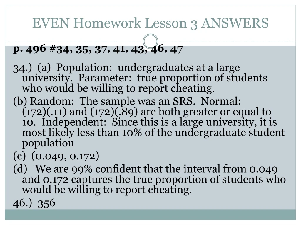
EVEN Homework Lesson 3 ANSWERS. p. 496 #34, 35, 37, 41, 43, 46, 47 34.) (a) Population: undergraduates at a large university. Parameter: true proportion of students who would be willing to report cheating.

E N D
EVEN Homework Lesson 3 ANSWERS p. 496 #34, 35, 37, 41, 43, 46, 47 34.) (a) Population: undergraduates at a large university. Parameter: true proportion of students who would be willing to report cheating. (b) Random: The sample was an SRS. Normal: (172)(.11) and (172)(.89) are both greater or equal to 10. Independent: Since this is a large university, it is most likely less than 10% of the undergraduate student population (c) (0.049, 0.172) (d) We are 99% confident that the interval from 0.049 and 0.172 captures the true proportion of students who would be willing to report cheating. 46.) 356
Unit 8 Lessons 4 and 5 Estimating a population mean Section 8.3
OBJECTIVES Construct and interpret a confidence interval for a population mean. Determine the sample size required to obtain a level C confidence interval for a population mean with a specified margin of error. Carry out the steps in constructing a confidence interval for a population mean: define the parameter; check conditions; perform calculations; interpret results in context. Determine sample statistics from a confidence interval Understand why each of the three inference conditions – Random, Normal, and Independent – is important.
One-Sample z Interval for a Population Mean • Statistic ± (critical value) • (standard deviation of statistic) • Let’s rewrite this specifically for the population mean: • This is from an SRS of size n from a large population that contains an unknown mean µand KNOWN standard deviation σ. As long as the Normal and Independent conditions are met, z* is the critical value for the standard Normal curve with area C between –z* and z*. • This interval is sometimes called a one-sample z interval for a population mean.
Choosing the Sample Size • When you start planning a study, you might be unsure how large of a sample you want, but you might have an idea of the margin of error you want it to be/keep below. • Recall the confidence interval for estimating a population’s mean • If we want to keep it within a specific margin of error, we can set up an inequality that would look like this: This part represents your margin of error
Choosing the Sample Size • We will have to guess the . • Get a reasonable value by using a standard deviation from a pilot study/past experience with similar studies . Wait, how do we know the population’s standard deviation? This critical value will be determined by the Confidence level (given to you in the problem) This n is what we want to solve for!
EXAMPLE Administrators at your school want to estimate how much time students spend on homework, on average, during a typical week. They want to estimate µ at the 90% confidence level with a margin of error of at most 30 minutes. A pilot study indicated that the standard deviation of time spent on homework per week is about 154 minutes. How many students need to be surveyed to estimate the mean number of minutes spent on homework per week with 90% confidence and a margin of error of at most 30 minutes? The administrators need to survey at least 286 students.
What if the standard deviation is unknown??? Most of the time, if you don’t know the population mean, you’re not going to know the population standard deviation either! Recall that if the sampling distribution of is approximately Normal, we can find probabilities involving by standardizing: Since we typically don’t know the standard deviation, we can use the standard deviation of our sample:
ACTIVITY: BINGO! • If we are doing inference about a population mean µ, what happens when we use the sample standard deviation sx to estimate the population standard deviation σ? • Before we look into this, let’s look at a population we might know more information about: • Let’s start with a Normal population with mean µ=100 and standard deviation σ = 5. • We are going to take an SRS of size 4 from the population; • We are going to compute the sample mean • Standardize the value of the sample mean using the “known” value σ = 5. • In your calculator, this is what you will type: randNorm(100, 5, 4)L1: 1-Var Stats L1: ( -100)/(5/√4) Math PRB option 5 STO> LIST (2nd STAT) L1 : (ALPHA .) STAT Calc option 1 : (ALPHA .) VARS 5: Statistics option 2
ACTIVITY: BINGO! Hit Enter 100 times and say BINGO every time your z-score is above 3 or below -3 standard deviations Write down the value every time you say BINGO According to the 68-95-99.7 rule, about how often should a “Bingo!” occur?
ACTIVITY: BINGO! • Now let’s see what happens when you standardize the value of using the sample’s standard deviation sxinstead of the “known” σ. • In your calculator, this is what you will type: • ENTRY (2nd ENTER) … this pulls up what you previously typed • You want to change the standard deviation of 5 to the sample’s standard deviation sx . • To do this: Using the arrow keys, scroll to the last command and put your cursor on 5, then hit VARS option 5: Statistics option 3:Sx • AGAIN, Hit Enter 100 times and say BINGO every time your z-score is above 3 or below -3 standard deviations • Write down the value every time you say BINGO.
ACTIVITY: BINGO! What did you notice the difference between when we used the POPULATION’S standard deviation σ versus when you used the SAMPLE’S standard deviation sx? There were more Bingos the 2nd time – meaning that there were more z-scores outside of 3 standard deviations. – way more than 0.03%. What does this mean?!?
t distribution • When we used our sample’s standard deviation, what happened? • More values were outside 3 standard deviations! • This is representing a NEW distribution: the t distribution: • It has a slightly different shape than the standard Normal curve - it’s still symmetric with a single peak, but with much more area in the tails. • See page 504 in your textbook to see a picture of the shape differences
William S. Gosset (1876 – 1937) This distribution was discovered by William S. Gosset, who worked for the Guinness Brewery – his goal in life was to make better beer. He found that when using small samples, his quality tests weren’t quite right, but then took time off to study the problem, and eventually discovered the new model, calling it the “t” distribution He used his new t procedures to find the best combination of barley and hops, which got him the job of head brewer. Guinness didn’t provide much support for the work. Gosset used the penname “Student” when publishing this mathematical work, so often the t distribution is referred as the “Student’s t”.
Degrees of Freedom The statistic t has the SAME interpretation as any standardized statistic: it says how far is from its mean in standard deviation units. There is a different t distribution for each sample size. Because of this, we need to identify a particular t distribution by number of degrees of freedom (df ) df = n – 1 (subtract 1 from the sample size) The notation to identify a t distribution with a particular degrees of freedom is tn-1
The t distributions, Degrees of Freedom Draw an SRS of size n from a large population that has Normal distribution with mean µ and standard deviation σ. The statistic: Has the t distribution with degrees of freedom df= n-1. The statistic will have approximately a tn-1 distribution as long as the sampling distribution is close to Normal.
More about the Degrees of Freedom • The density curves of t distributions are similar in shape to the standard Normal curve • The spread of t distributions is a bit greater than that of the standard Normal distribution. • As the degrees of freedom increase, the t density curve approaches the standard Normal curve more closely. • This is because the larger the sample size, the closer your sx gets to σ.
Using TABLE B Table B shows the critical values t* for the t distributions. The left column represent the degrees of freedom Common confidence levels are given at the bottom of the table. By looking down any column, you can check that the t critical values approach the Normal critical values z* as the degrees of freedom increase.
EXAMPLE - Using TABLE B Suppose you wanted to construct a 90% confidence interval for the mean µ of a Normal population based on an SRS of size 10. What critical value t* should you use? Using the line for df = 10 -1 = 9 and the column with a tail probability of .05 (10%/2), the desired critical value is t* = 1.833.
YOUR TURN Use Table B to find the critical value t* that you would use for confidence interval for a population mean µ for a 98% confidence interval based on n=22 observations. Using the line for df = 22 -1 = 21 and the column with a tail probability of .01 (2%/2), the desired critical value is t* = 2.518.
In your calculator • For TI-84: • DISTRIBUTION (2nd VARS), option 4: invT( • In the parentheses, type in the area to the left of the desired critical value, the degrees of freedom. • From the last problem, you would type in invT(.01,21)
CONTRUCTING A CONFIDENCE INTERVAL FOR µ • First, check your conditions! • RANDOM: The data comes from a random sample of size n from the population of interest of a randomized experiment. • NORMAL: The population has a Normal distribution of the sample size is large (n≥30). • INDEPENDENT: 10% rule: The sample size is no more than 1/10 of the population.
The One-Sample t Interval for a Population Mean Estimate ± (critical value)(standard deviation of statistic) Remember, technically we call the standard error of the sample mean – which describes how far will be from µ on average, in repeated SRSs of size n.
EXAMPLE As part of their final project in AP Statistics, Christina and Rachel randomly selected 18 rolls of generic brand of toilet paper to measure how well this brand could absorb water. To do this, they poured ¼ cup of water onto a hard surface and counted how many squares it took to completely absorb the water. Here are the results from their 18 rolls: 29 20 25 29 21 24 27 25 24 29 24 27 28 21 25 26 22 23 Construct and interpret a 99% confidence interval for µ = the mean number of squares of generic toilet paper needed to absorb ¼ cup of water.
EXAMPLE STATE: We want to estimate µ = the mean of number of squares of generic toilet paper needed to absorb ¼ cup of water with 99% confidence.
EXAMPLE • PLAN: We will construct a one-sample t interval, provided the following conditions are met: • RANDOM: The students selected the rolls of generic toilet paper at random. • NORMAL: Since the sample size is small (n=18), and we aren’t told that the population is Normally distributed, we need to check whether it is reasonable to believe that the population has Normal distribution. (draw a dotplot to see that there are no outliers and it roughly follows a Normal distribution) • INDEPENDENT: Since we are sampling without replacement, we must check the 10% condition. It is reasonable to believe that there are at least 10(18) = 180 rolls of generic toilet paper.
EXAMPLE DO: The sample mean for these data is and the sample standard deviation is . Since there are 18 – 1 = 17 degrees of freedom and we want 99% confidence, we will use a critical value of t* = 2.898 (from Table B).
EXAMPLE CONCLUDE: We are 99% confident that the interval from 22.99 squares to 26.89 squares captures the true mean number of squares of generic toilet paper needed to absorb ¼ cup of water.
Using t Procedures Wisely • What happens when a condition for using a t procedure is violated?? • If your result is still pretty accurate, then we call that procedure ROBUST. • According to the Merriam Webster Dictionary, a definition for robust “is having or showing vigor, strength, or firmness”….or another one is “capable of performing without failure under a wide range of conditions “ • According to Statistics, an inference procedure is robust if the probability calculations involved in that procedure remain fairly accurate when a condition for using the procedure is violated.
Using t Procedures Wisely • Good news for us! • The t procedures are quite robust against non-Normality of the population EXCEPT when outliers or strong skewnessis present. • Larger samples improve the accuracy of critical values from the t distributions when the population is not Normal because: • The sampling distribution of is close to Normal if the sample size is large enough (CLT!) • As the sample n grows, the sample standard deviation sx will be an accurate estimate of σ whether or not the population has Normal distribution.
Using t Procedures Wisely • Always plot the data to check if it’s roughly Normal – but more importantly, that there’s no outliers or major skewness. • And it’s definitely MORE important to make sure that it comes from RANDOM data, rather than being picky about how Normal it looks. • Follow these procedures to help using sample size n: • If n<15: Use t procedures if the data appears close to Normal (roughly symmetric, single peak, no outliers). If the data are clearly skewed or there are outliers, DO NOT USE t. • If n≥15: The t procedures can be used except in the presence of outliers or strong skewness. • Large samples (n≥30): The t procedures can be used even for clearly skewed distributions when the sample is large!
EXAMPLE – can we use t? • Don’t use t for these situations either: • If your sample data gives a biased estimate for some reason • And if you have all the data for all your population of interest • Determine whether we can safely use a one-sample t interval to estimate the population mean in each of the following settings: • A.) Below is a histogram of the total number of students in class and their heights. NO. We have data for the entire number of students, so we do NOT need inference. Remember, you only use inference when you are ESTIMATING something about the population (because that proportion or mean is unknown!)
EXAMPLE – can we use t? • Determine whether we can safely use a one-sample t interval to estimate the population mean in each of the following settings: • B.) The dot plot below shows expenditure costs for 6 of the employees at a company NO. This is a sample of 6 (less than 15!), so we can only use t procedures if the data appears close to Normal. It does not appear that way.
EXAMPLE – can we use t? • Determine whether we can safely use a one-sample t interval to estimate the population mean in each of the following settings: • C.) The boxplot below shows the SAT Math scores for a random sample of 20 students at your high school. YES. The sample size is 20 (greater than 15!) Although slightly skewed, there doesn’t seem to be strong skewness or the presence of any outliers. For more examples with these, see p. 513 in book
In your calculator: • One-sample t intervals for µ on your calculator: • STAT TESTS option 8:Tinterval… • If the problem gives you actual data: • (Make sure your data is in L1) Choose Data option, List:L1, Freq:1, C-level: (type in your confidence level out of percent form), Highlight Calculate and press ENTER • If the problem just gives you summary statistics: • Choose Stats option, and type in your sample mean, sample standard deviation, sample size n, and C-level (out of percent form), Highlight Calculate and press ENTER • Calculators aren’t always right! Be careful because sometimes there are called “parallel solutions” where your calculator and your calculations might give you two different answers. That’s why you always need to show your work and explanation on exams!
EXAMPLE – for practice! • The principal at a large high school claims that students spend at least 10 hours per week doing homework, on average. To investigate this claim, an AP Statistics class selected a random sample of 250 students from their school and asked them how long they spent doing homework during the last week. The sample mean was 10.2 hours and the sample standard deviation was 4.2 hours. • (a) Construct and interpret a 95% confidence interval for the mean time that students at this school spent doing homework in the last week. • (b) Based on your interval in part (a), what can you conclude about the principal’s claim?
EXAMPLE STATE: We want to estimate µ = the mean time spent doing homework in the last week for students at this school with 95% confidence.
EXAMPLE • PLAN: We will construct a one-sample t interval, provided the following conditions are met: • RANDOM: The students were randomly selected. • NORMAL: We are not told if the population is normal. However, since the sample size is large (n=250), we are safe using t procedures. • INDEPENDENT: Since we are sampling without replacement, we must check the 10% condition. It is reasonable to believe that there are at least 10(250) = 2500 students since it is a large high school.
EXAMPLE DO: The sample mean for these data is and the sample standard deviation is . Since there are 250 – 1 = 249 degrees of freedom and we want 95% confidence, we will use a critical value of t* = 1.984 (from Table B).
EXAMPLE CONCLUDE: We are 95% confident that the interval from 9.67 hours to 10.73 hours captures the true mean of hours that students at this school spent doing homework in the last week. (b) Since the interval of plausible values for µ includes values less than 10, the interval does not provide convincing evidence to support the principal’s claim that students spend at least 10 hours on homework per week, on average.
Lesson 4: Homework problems Complete online notes. Read textbook pages: p. 499-511 Complete exercises: p. 518 #55, 57, 59, 60, 63 Check answers to odd problems
Lesson 5: Homework problems Read textbook pages: p. 511-517 Complete exercises: p. 519 #65-67, 71, 73-78 Check answers to odd problems