Download
1 / 56
570 likes | 717 Views
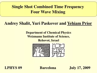
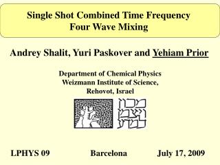
Single Shot Combined Time Frequency Four Wave Mixing. Andrey Shalit, Yuri Paskover and Yehiam Prior. Department of Chemical Physics Weizmann Institute of Science, Rehovot, Israel. LPHYS 09 Barcelona July 17, 2009.

E N D
Single Shot Combined Time Frequency Four Wave Mixing Andrey Shalit, Yuri Paskover and Yehiam Prior Department of Chemical Physics Weizmann Institute of Science, Rehovot, Israel LPHYS 09 Barcelona July 17, 2009
Molecular spectroscopy can be performed either in the frequency domain or in the time domain. • In the frequency domain, we scan the frequency of excitation (IR absorption), or the frequency of observation (Spontaneous Raman spectroscopy), etc. • Alternatively, we can capture the time response to impulse excitation, and then Fourier Transform this signal to obtain a frequency domain spectrum. • We are always taught that the choice of one or the other is a matter of convenience, instrumentation, efficiency, signal to noise, etc. but that the derived physical information is the same, and therefore the measurements are equivalent.
Outline • Time Frequency Detection (TFD) : the best of both worlds • Single Shot Four Wave Mixing • Tunable Single Shot Four Wave Mixing • Multiplex Single Shot Four Wave Mixing • TFD simplified analysis • Conclusions
Outline • Time Frequency Detection (TFD) : the best of both worlds • Single Shot Four Wave Mixing • Tunable Single Shot Four Wave Mixing • Multiplex Single Shot Four Wave Mixing • TFD simplified analysis • Conclusions
Spontaneous Raman spectrum of CHCl3 Direct spontaneous Raman spectrum (from the catalogue)
Dk w1 w1 k2 kCARS w2 wAS k1 k1 WRaman 2w1- w2- wAS = 0 Coherent Anti Stokes Raman Scattering (CARS) Conservation of Momentum (phase matching) Energy conservation Dk = 2k1-k2-kAS= 0
Time Resolved Four Wave Mixing • A pair of pulses (Pump and Stokes) excites coherent vibrations in the ground state • A third (delayed) pulse probes the state of the system to produce signal • The delay is scanned and dynamics is retrieved
Ea Eb Ec Time delay Time Resolved Four Wave Mixing Phase matching ~ 50-100 femtosecond pulses ~ 0.1 mJ per pulse
Time Domain vs. Frequency Domain In this TR-FWM the signal is proportional to a (polarization)2 and therefore beats are possible
Time frequency Detection (CHCl3) Open band: Summation over all frequencies (Δ)
F.T Open band:
Limited Band Detection Summation over 500cm-1 window
Open vs. Limited Detection F.T Open band: F.T Limited band:
Spectral Distribution of the Observed Features 104 cm-1 365 cm-1 Observed frequency: 104 cm-1 Observed detuning : 310 cm-1 Observed frequency: 365 cm-1 Observed detuning : 180 cm-1
However, this is a long measurement, it takes approximately 10 minutes, or >> 100 seconds. In what follows I will show you how this same task can be performed much faster. 1015 times faster, or in < 100 femtoseconds !
Outline • Introduction, or “TFD: the best of both worlds” • Single Shot Four Wave Mixing • Tunable Single Shot Four Wave Mixing • Multiplex Single Shot Four Wave Mixing • TFD simplified analysis • Conclusions
Spatial Crossing of two short pulses:Interaction regions k3 k1 k3 arrives first k1 arrives first 100 fsec = 30 microns 5mm Beam diameter – 5 mm Different regions in the interaction zone correspond to different times delays
k2 z k3 k1 k1 k3 x k2 ks y CCD Three pulses - Box-CARS geometry Time delays Spatial coordinates
k2 k1 k3 Pump-probe delay z -y +y k1 first k3 first k2 k1 k3 Pump-probe delay Intersection Region: y-z slice
CH2Cl2 Single Pulse CARS Image
CHBr3 Several modes in the range
Outline • Introduction, or “TFD: the best of both worlds” • Single Shot Four Wave Mixing • Tunable Single Shot Four Wave Mixing • Multiplex Single Shot Four Wave Mixing • TFD simplified analysis • Conclusions
k2 z k3 k1 k1 k3 x k2 ks y CCD x y z Geometrical Effects
Spectrum of the central frequency (coherence peak) as a function of the Stokes beam deviation
Measured and calculated tuning curve Measured Calculated
For each time delay, a spectrally resolved spectrum was measured.
Outline • Introduction, or “TFD: the best of both worlds” • Single Shot Four Wave Mixing • Tunable Single Shot Four Wave Mixing • Multiplex Single Shot Four Wave Mixing • TFD simplified analysis • Conclusions
k2 z k3 k1 k1 k3 x k2 ks y CCD Single Shot Geometry: Parallel beams
Single Shot Geometry: Focused Beam z x y k1 k3 k2 CCD L
k2 k1 k3 Pump-probe delay z -y +y k1 first k3 first k2 k1 k3 Pump-probe delay Intersection Region: y-z slice
Intersection Region: y-z slice z -y +y k1 first k3 first
Intersection Region: y-z slice z -y +y Δ
τ [fs] Δ Time Frequency Detection:Multiplex single Shot Image Focusing angle : δ = 3 mrad (CH2Br2)
Outline • Introduction, or “TFD: the best of both worlds” • Single Shot Four Wave Mixing • Tunable Single Shot Four Wave Mixing • Multiplex Single Shot egenerate Four Wave Mixing • TFD simplified analysis • Conclusions
k3 k3 k1 -k2 + -k2 k1 Time Frequency Detection 0 Detuning from a probe (k3) carrier frequency
Spectral Distribution of the Signal Produced by a Fundamental Mode In TR-DFWM, we have shown that because of the quadratic dependence on the polarization, fundamental modes may be seen only after linearization of the signal, i.e. by heterodyne detection 0 Detuning from a probe carrier frequency (Δ)
Spectral Distribution of the Signal Produced by Intensity Beat 0 Detuning from a carrier (Δ)
Identification of signals: Fundamental modes of frequency Ω1 are spectrally peaked at Ω1/2 Intensity beats at frequency (Ω1 ± Ω2) spectrally peaked at [ (Ω1-Ω2)/2 ] Based on this result, it is now possible to directly and unambiguously identify the character of each peak